
Neighborhood Effect, Agricultural Development and Poverty Level in Nigeria
- Oluwatobi Joshua OLOFIN
- Adeleke Gabriel AREMO (Ph.D)
- Olabode Philp OLOFIN (Ph.D)
- Oluwafemi Olawale OKUNADE
- 705-726
- Jun 7, 2023
- Agriculture
Neighborhood Effect, Agricultural Development and Poverty Level in Nigeria
Oluwatobi Joshua OLOFIN1, Adeleke Gabriel AREMO (Ph.D) 2, Olabode Philp OLOFIN (Ph.D) 2, Oluwafemi Olawale OKUNADE2
1Department of Economics, Universität Göttingen, Göttingen, Germany
2Department of Economics, Obafemi Awolowo University, Ile-Ife, Nigeria
DOI: https://doi.org/10.47772/IJRISS.2023.70557
Received: 31 March 2023; Revised: 18 April 2023; Accepted: 27 April 2023; Published: 07 June 2023
ABSTRACT
The study seeks to evaluate the role of agricultural development on poverty level and ascertain whether neighbouring countries have any influence on the relation between agricultural development and poverty level in Nigeria. Annual data covering the period between 1980 and 2019 were employed. Fully Modified Ordinary Least Square (FMOLS), Canonical Cointegrating Regression (CCR) and spatial econometrics were employed. Our results showed that agricultural development is capable of reducing poverty level in the country, while there was no significant effect of spatial factors on the relationship between agricultural development and poverty level in Nigeria between 1980 and 2019. The study therefore recommends that the government should pay more attention towards improvement of agriculture, transportation and oil rent which are capable of complementing each other in reducing poverty in Nigeria.
Keywords: Agricultural development; Poverty; Neighborhood effect; Nigeria.
INTRODUCTION
Although, Nigeria is blessed with good climate and free natural resources suitable enough to drive primary sector of her economy, she is one of the countries that are not likely to meet the United Nations’ Sustainable Development Goal (SDG) of ending extreme poverty by 2030. According to World Poverty Clock (2019), in terms of poverty level, Nigeria has overtaken India whose population is about seven times larger and has become the most extreme poor country in the world. Based on facts from National Bureau of Statistics (2020), 40.1% (83 million) Nigerians are considered poor by national standards, with Sokoto, Taraba and Jigawa states being the poorest.
In the 60’s, the main stay of the economy is agriculture which provides employment for more than 60% of the population and generates more than 70% of the country’s revenue. After the discovery of oil in the 70’s, there was a total shift from agriculture to oil sector. Unfortunately, employment generating capacity of oil sector is very low compared to agricultural sector. One thing that is also obvious from oil sector revenue is that, it is very easy for a few privileged Nigerians to pocket most of the oil sector’s revenue without been noticed. This has promoted corruption alongside total neglection of agricultural funding and caused huge reduction in the country’s revenue. This reduction in revenue, coupled with sharp increase in government expenditure, as well as a high level of corruption had denied the government the ability to cater for the needs of the Nigerians (Anfofum and Olure-Bank, 2018). Poverty level keeps increasing due to government inability to fund parastatals, pay workers’ salaries promptly and servicing debt. This has led the government to pay new attention to the long-neglected agricultural sector with the aim of increasing food supply which is expected to lower food prices as well as reducing poverty level in the country.
Various agricultural programmes such as National Accelerated Food Production Programme (NAFPP) (1972-1973), Operation Feed the Nation (OFN) (1976-1980) and Green Revolution Programme (GRP) (1981-1983) have been implemented to resuscitate agricultural sector in Nigeria. Also, some agency-based intervention programmes such as National Agricultural Land Development Authority (NALDA), River Basin Development Authority (RBDA), Agricultural Development Programmes (ADPs), Directorate of Food, Road and Rural Infrastructure (DFRRI), Anchor Borrowers Programme, launched in 2015 and the Green Imperative Programme, launched in 2020 were put in-place. Despite all the above programmes and interventions, the level of poverty in Nigeria keeps rising, especially in the Northern region of the country (Ngbea and Achunike, 2014). The question now is whether or not agricultural development can actually reduce poverty level in Nigeria.
Many studies have been done on the contributions of agricultural development to poverty reduction worldwide. The findings of these studies lack empirical generality. Majority of these studies support substantial benefits of agricultural development to poverty reduction, especially in developing countries such as Nigeria where favourable climatic condition exists (Christiansen, et al. 2010; Umaru and Zubairu (2012). Unfortunately, few studies, if exists, have studied the role of country’s location on the connection between agricultural development and poverty level in Nigeria. Recently, it has been proved that whatever happens to a country may be correlated with whatever happens in other countries, regions or nearby neighbours. According to Le Sage (2008), conventional growth regressions assume independent regional observations, but there is a growing consensus that regional income growth rates exhibit spatial dependence. It has been noted by Ramirez and Loboguerrero (2002) that spatial effects are important in explaining economic growth since countries can interact with each other through technological diffusion and capital inflows as well as common political, economic and social policies. Thus, spillover effects among the neighbouring countries can contribute to growth and development. Controlling for spatial dependence in a growth model can help in determining whether economic growth in one country is affected by or related to the economic growth rate of its neighbouring countries. This notion is likely to be unavoidable in developing countries, especially in Nigeria (where poverty is highly endemic) that is surrounded by agrarian and poor countries. Success or failure of these countries in terms of agricultural development and poverty reduction can have substantial effect on development programmes in Nigeria.
On this note, this study seeks to add to knowledge by investigating the potential of agricultural development towards poverty reduction, as well as determine whether or not the failure of agricultural development in the past has anything to do with spatial dependence (i.e. whether the situation in Nigeria’s neighbouring countries have any impact on the relationship between agricultural development and poverty level in Nigeria or not). This article is divided into five sections. The second section reviews the empirical literature, the third section presents the theoretical framework, the fourth section explains the methodology and finally, the fifth section discusses the results and suggests policy recommendations.
REVIEW OF EMPIRICAL LITERATURE
The role of agricultural sector in terms of income generation to the extreme poor compared to other sectors of the economy cannot be overemphasized (Townsend, 2015). Noted in the literature is that, as economy improves, a predictable consequence is a reduction in the contribution of agriculture to national employment and Gross Domestic Product (Timmer, 1988; Byerlee, De Janvry and Sadoulet, 2009; Brooks et al., 2009). Unfortunately, this is not the case in Nigeria and many other developing countries. This could be associated with greater income elasticities of demand for non-agricultural products. As income of consumers rises, they consume more of manufactured goods and services at a rate higher than their consumption of food. One paradox however, is that this usually leads to increasing incomes and lower levels of poverty among people who rely on agriculture for a living. On a global level, this may lead countries that focus on growth of the agricultural sector to perform better than countries that focus on other sectors.
Cervantes-Godoy and Dewbre (2010) explained why some countries are performing better than others, by examining shared features of twenty-five countries where extreme poverty has been drastically reduced over the past twenty to twenty-five years before the time of the study. The basis of comparison of these countries was some macroeconomic indicators, especially their agricultural economic features. The selected countries adequately represented all geographic regions, not tilting towards the richest or poorest countries, and also included countries with diverse systems of government, notwithstanding whether their macroeconomic and agricultural economic performances were similar. The study discovered that despite that economic growth influenced fall in poverty, the growth of different sectors, especially growth in agricultural income was the most important. Majority of the poor in Nigeria participate in agriculture (Mbam and Nwibo, 2013), which has been able to reduce poverty in countries like China, Mexico and India (Ogbalubi and Wokocha, 2013), yet poverty keeps on rising in Nigeria.
Christiaensen and Demery (2007) posited that, what economic growth contributes to poverty reduction level might vary across sectors, since poor people may easily be able to obtain the benefits of growth if growth occurs in the region where they are located. What this suggests, is that because of market segmentations and consideration of political economy, income generated in one geographical location or economic sector cannot be easily transferred to another economic location or sector. The study also discovered that growth emanating from the agricultural sector has more influence on poverty reduction than growth emanating from non-agricultural sectors. Similarly, Ravallion and Montalvo (2009) found out that the primary sector was mainly responsible for China’s victory over poverty as opposed to the secondary and tertiary sector of the economy. In China, the growth in the agricultural sector was able to reduce poverty at quadruple the rate at which growth in the industry and service sectors could reduce poverty, because of relative equality in land distribution. The impact of a rising agricultural sector was however less in India and Pakistan, because of unequal distribution of resources (Christansen et al, 2010).
Examining the role agriculture plays in reducing poverty, Christansen et al (2010) stated that how much a sector of the economy will influence poverty level is determined not only by the performance of such a sector, but also how the sector affects other sectors, the rate of involvement of poor people in the sector and how large it is. Using cross-country econometric evidence to pool these effects together, they discovered that agricultural sector had more effect than non-agricultural sector in poverty reduction among the extremely poor. In addition, the agricultural sector is up to 3.2 times more potent in reducing the population of those who live on less than $1 per day in countries with low income and abundant resources (including sub-Sahara African countries). The non-agricultural sector was only found to be better at poverty reduction in the midst of the better-off poor (those living on more than $1 but less than $2 per day).
Most of the people living in sub-Saharan Africa live in rural regions, where there are more extreme cases of poverty. Because almost all rural households depend on agriculture and considering the huge impact of the agricultural sector on the overall economy, it seems agriculture should definitely be a vital sector to economic development. However, even though agricultural-led growth has helped in reducing poverty in many Asian countries, this has not been the case in Africa (Diao et al., 2010).
One area in which many poverty appraisals lag behind is in terms of differentiating between poor groups and other parameters aside from income. Little emphasis is placed on the relationships between poverty level and geographical location. The information they do provide is about, who is regarded as poor and the nature of poverty, but studying spatial patterns of poverty can help to explain the causes of poverty (Henninger, 1998). Only few recent studies consider the basis that economic units with similar features are at times clustered together by choice or because of a forceful influence of economic, political or social reasons (Voss et al, 2006). Advancement in spatial analytical techniques have made it possible to identify these households and measure spatial patterns of poverty (Sowunmi et al, 2012). It is very important to study spatial determinants with regards to natural resources because natural capital asset holdings are difficult to describe with conventional variables but are distributed across geographical locations. Because of little access to relevant information, geographical targeting has many advantages over other targeting methods. Targeting methods directed at poverty reduction and based on geography are mainly used because wide differences exist in living standards across geographical regions and poverty is concentrated in some of these regions (Bigman & Fofack, 2000).
According to Farrow et al (2005) in their study on how food poverty and food consumption are distributed, using statistical and spatial analysis and generated hypothesis of food poverty estimates in districts of Ecuado, it was discovered that the food poor were clustered in certain regions and a substantial number of them clustered in the Central Andean region. Using geographically weighted regression, it was established that the processes behind food poverty in Ecuador are spatially variable. Working on improving transport infrastructure was projected as a solution to reduce levels of food poverty in Ecuador, with the most benefit in the extreme southern district. The study did not focus on per capita expenditure, which is important because even though individuals may be able to afford food items, they may remain below the poverty line because of their inability to afford other basic items apart from food.
Also, Mindy and Bruce (2004), in an attempt to study spatial concentrations of poverty and poverty dynamics in the USA explained that poverty in USA is not distributed evenly across regions. The level of poverty in the rural counties and central cities were the highest and a cluster of poorer people was found in the isolated rural regions. Between 1990 and 2000, there was a decline in poverty from 13.1% to 12.4%, and this decline was especially in persistent poverty areas. The study did not state whether spatial concentrations of poverty had any effect on the poverty situation of the 1990’s or if the better economic situations were as a result of the changes in neighbouring areas.
Furthermore, using spatial regression techniques, Okwi et al (2006) observed the effects of geographic factors on poverty in Kenya and studied the relationship between poverty incidence and geographical conditions in rural Kenya. Results of the study showed, there were mixed effects of locational variables at national levels set against provincial levels. Differential influence of these variables and other factors at the location-level showed that provinces in Kenya are very heterogeneous. As a result of this heterogeneity, different spatial factors were considered necessary to explain welfare levels in different areas within the provinces. The study emphasized that investing in roads and improving soil fertility could reduce the level of poverty in Kenya.
The rural areas in Nigeria have significantly higher poverty rate than the urban areas and most residents of these rural areas rely heavily on agriculture for livelihood (FAO, 2006). As a result, investing in agricultural development in these regions is of utmost importance, since it could reduce their poverty rate drastically. This is buttressed by the work of Azuh and Matthew (2010) which employed the OLS method and cointegration test to examine the role of agriculture on poverty reduction and speeding-up economic development. The study discovered that all the identified agricultural prospects, represented with various variables are similarly important in improving the level of agricultural output in Nigeria within the period under study (1976-2004). The study gives further credence to the findings in empirical literature that agricultural development opportunities are especially sensitive in rural areas.
In conclusion, empirical literature shows that a large number of studies have been carried out on the relationship between agricultural development and poverty level in Nigeria, Africa and other regions of the world. Many focused specifically on certain regions in Nigeria (Olorunsanya et al., 2011; Amao et al, 2013; Adetayo, 2014; Oyhakilome and Zibah , 2014; Margwa et al, 2015). While these studies agree that poverty is more concentrated in rural areas, compared to the urban regions, they have ignored the influence of neighbouring regions (or country) on the relation between agricultural development and poverty level in Nigeria. This lacuna is expected to be filled in this article.
THEORETICAL FRAMEWORK
In the literature, there are mixed results on the role of agricultural development on poverty reduction, at least concerning the magnitude of its role. In the 1960s and 1970s, agriculture has been noted to be a backward subsistence sector compared to its counterpart, the industrial sector (Lewis, 1954). This has led to interpreting early development economics as supporting industrialization strategy as more vibrant, resulting in an “urban bias” in development planning (Lipton, 1977). Contrary to the above, after the seminal work of Johnston and Mellon (1961) and Schultz (1964), It was noted that, even though agriculture might not grow as fast as non-agricultural sector, it might lead to faster overall economic growth and this notion has been confirmed by many studies (Haggblade, Hammer and Hazell, 1991; Delgado et al., 1998).
Developing countries like Nigeria are characterized by income disparities between urban and rural sectors and these inequalities in income are highly important in the overall inequality situation of such countries (Fields, 1980; Bourguignon and Morrison, 1990). Ravillion and Datt (1999) outlined a simple dual sector (or two-sector) economy theory, based on the dual sector model of W. Arthur Lewis (Lewis, 1954). In this model, poverty reduction is captured in the form of absorption of poor agricultural-sector workers into the non-poor non-agricultural sector. The theory assumes that any agricultural worker who wants to participate in non-agricultural sector activities incurs a cost in doing that. This cost determines the equilibrium differential earnings between the agricultural sector and the non-agricultural sector. This cost incurred eventually leads to a reduction in overall output. Also, this cost leads to a fall in the absorption of labour into the non-agricultural sector. Recently, attention has shifted towards the contribution of agriculture to poverty reduction since economic growth does not necessarily imply poverty reduction, but the ability of the generality of people to partake from it. In developing countries, especially Africa, (Nigeria included), where majority of the population participate in agriculture, it is expected that participation effect is likely to be high. This then implies that participating effect is likely to be higher than overall economic growth effect in terms of poverty reduction. However, taking cognizance of economies of scale, it should also be noted that only large commercial farmers may enjoy the participation effect of African agricultural development program, while majority of the poor small farm owners may not. Thus, the extent to which agriculture can benefit majority of the poor in terms of poverty reduction is questionable.
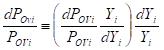
Given this fact, suppose we make a (decomposable) measure of poverty and per capita Gross Domestic Product (GDP) in a country , we can consider the proportionate change in poverty in this country identical to the GDP elasticity of poverty (the proportionate change in poverty divided by the proportionate change in GDP per capita), multiplied by the proportionate change in GDP per capita ( ):
 (1)
(1)
where the first multiplicative term in equation (1) is referred to as the participation effect while the second multiplicative term is the growth effect. According to the World Bank (2000), it is neither all the growth practices that bring about equivalent inclusive growth, nor an equal extent of poverty reduction. This implies that growth effects and participation effects may vary significantly through sectors. Differences in participation effect have been examined by different studies such as the one done for India by Ravallion and Datt (1996; 2002) and for China by Ravallion and Chen (2004).
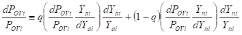
To incorporate these variations, we can rewrite equation (1) as weighted sum of the contributions of both the agricultural and the non-agricultural sectors to poverty reduction as:
 (2)
(2)
where denotes “agriculture”, equals “non-agriculture”, and equals “any constant (1<q<0 )”. An expressive choice for q can be given as q= (Yai/Yi)=sai the portion of agriculture in total GDP in country . This then follows that (1-q) equals (Ym/Yi)=sm , the portion of non-agriculture in total GDP in country i. Thus, equation (2) turn out to be:
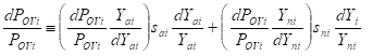 (3)
(3)
Representing rates of change for POVi and Yi with lower case gives:
![]() (4)
(4)
where yki is “the growth rate of per capita GDP” k= a, n, εki in sector “the elasticity of total poverty with respect to per capita GDP in sector k ”, ski and “the share of sector in total GDP”.
From equation (4), we can show that the influence of each sector (e.g. agriculture) on poverty is dependent on how its growth affects poverty, in comparison to the other sector (non-agricultural sector such as manufacturing). Also, many studies have shown how improved agricultural growth can spur changes in other sectors of the economy, and how these changes can cause increased growth in other non-agricultural sectors. Even though, the possibility of having reverse interaction of the above has been noted, the literature noted that these effects are not much. Considering the above therefore suggests that the growth effect of a sector could have both direct effect (size of ya ) and an indirect effect, which could be any other changes in poverty due to change in the growth effect of other sector (the effect of ya on yn ). More so, it is argued here that an equivalent improvement in the pace of per capita agricultural growth (ya ) is likely to have higher effect on poverty level than an identical increase in the rate of non-agricultural growth (yn ), if εn sn<εa sa
Overall from the above, we can deduce that participation effect has two elements which are: (i) elasticity constituent and (ii) a share constituent. In most developing countries, agriculture is the largest sector in the economy, but its share is the lowest compared to the portion of non-agriculture (services and industry combined). However, whether the participation effect of agriculture (εa sa ) overshadows the participation effect of non-agriculture (εn sn ) would be dependent on whether εa is satisfactorily larger than εn and when εa=εn, equation (4) collapses to equation (1) “and the source of growth no longer matters in the determination of the poverty effect of growth” (Ravallion and Datt, 1996).
Model Specification of the impact of agricultural development on poverty level in Nigeria
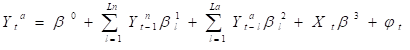
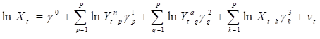
To specify the relationship between agricultural development and poverty level in Nigeria, if the above explanation is considered, we can assume that non-agricultural GDP per capita ( Ynt) in the country at time t depends on both the levels of per capita non-agricultural GDP in previous periods and the per capita agricultural GDP at present period. More so, if we consider a vector Xt of exogenous explanatory factors, we can have:
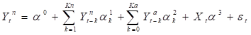 (5)
(5)
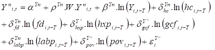
Similarly, we can represent per capita agricultural GDP as:
 (6)
(6)
Where Xt consists of human capital (hc), financial deepening (fd), health expenditure (hxp), manufacturing sector (manuf), transportation (transp), oil rent (oilrent), control of corruption (corpc), government effectiveness (goveff), regulatory quality (reguq) and poverty (pov). εt and ϕit are white noise error terms. We assume that equation (5) and (6) capture the full correlations between (per capita) non-agricultural and agricultural GDP. Thus, and εit and ϕit are assumed to be uncorrelated. These equations consist of intersectoral growth linkages, where agricultural and non-agricultural GDP are interdependently determined in a dynamic process. Substituting equation (6) into equation (5), we have a compact form equation for non-agricultural growth as:
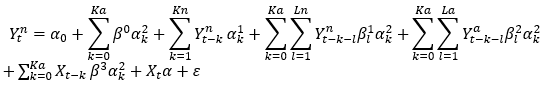 (7)
(7)
Equation (7) can further be reduced to:
 (8)
(8)
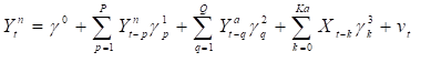
Now, this single equation establishes a dynamic relationship between non-agricultural GDP and the lagged levels of agricultural and non-agricultural GDP, and can be estimated with the use of Fully modified ordinary least square (FMOLS) and Canonical Cointegration Regression (CCR). To use the FMOLS and CCR, we need our Vector Autoregressive (VAR) lag order. In a VAR model, all the variables must have equal number of lags, which will be determined by finding the optimal lag (P). This is shown from equation (9) to (11)
 (9)
(9)
 (10)
(10)
 (11)
(11)
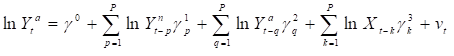
On the basis of the VAR model results, cointegrating regression is estimated. Cointegrating equations can provide a check for robustness of results and are able to produce reliable estimates in small sample size. If the series are cointegrated at first difference ‘I(1)’, Fully Modified Ordinary Least Square (FMOLS) is suitable for estimation. FMOLS according to Philips and Hansen (1990) gives optimal estimates of cointegrating regressions. FMOLS modifies least squares to explain serial correlation effects and for endogeneity in the regressors that comes from the presence of a cointegrating relationship.
![]() (12)
(12)
![]() (13)
(13)
![]() (14)
(14)
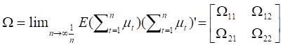
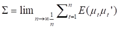
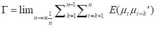
Where d1t and d2t are deterministic trend regressors. d1t enters both the cointegrating equation and the regressors equations while d2t enters only the regressors equations. u1t is the cointegrating equation error, while u2t are regressors innovations. If innovation ut =(u1t , u2t) are strictly stationary and ergodic with zero means, contemporaneous matrix , Σ one-sided long-run covariance (LRCOV) matrix Λ and non-singular LRCOV matrix Ω :
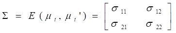 (15)
(15)
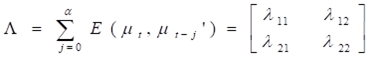 (16)
(16)
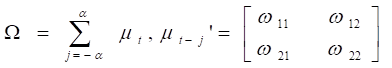 (17)
(17)
The Ordinary Least Square estimator now turns consistent with convergence at a rate quicker than the normal rate. If there is a “Long-run correlation” between u1t and u2t (ω12 ), or cross-correlation between the cointegration equation and the regression innovation λ12, Ordinary Least Square estimation will have an asymptotic distribution that is non-Gaussian, asymptotically bias, asymmetric and exhibition of non-scalar nuisance parameters. This shows that, conventional testing process will be void. This is where Fully-Modified Ordinary Least Square and Canonical Cointegration Regression (CCR) comes in, as they eradicate the asymptotic bias.
The Canonical Cointegration Regression (CCR) is based on a transformation of the variables in the cointegrating regression that removes the second-order bias of the OLS estimator in the general case. The long-run covariance matrix can be specified as:
 (18)
(18)
We can represent the matrix as:
![]() (19)
(19)
Where:
 (20)
(20)
 (21)
(21)
![]() (22)
(22)
The transformed series is obtained as:
![]() (23)
(23)
![]() (24)
(24)
The CCR takes the form below:
![]() (25)
(25)
where:
![]() (26)
(26)
Therefore, in this context, the OLS estimator of y1t*=β’y2t*+μ1t* is asymptotically equivalent to the ML estimator. This is because the transformation of the variables removes asymptotically, the endogeneity that is caused by the long-run correlation of y1t and y2t In addition, y1t*= μ1t-Ω12 Ω22(-1) μ2t shows how the transformation of the variables eliminates the asymptotic bias, due to the possible cross correlation between μ1t and μ2t.
Model Specification of neighbourhood effects on agricultural development and poverty level.
Spatial Lag Model.
To test for the spatial lag in this study, we take n to be “the number of countries” and W to be “the spatial weighting matrix of dimension (n × n)”, whose elements allocate “neighbours to each country” (Anselin, 1988). The weights matrix used can be described as W ={Wij} , such that 0 < Wij≤ 1 ∀i ≠ j, if I and j are neighbours, otherwise Wij= 0. Also, Wii= 0. We define countries as those that have a shared border. Using row-standardized weights (Anselin, 1988), Wi= 1. If we take equation (5) and (6) as the spatial lag model, it is expected that agricultural development (Ya(i,t) ) and the average income growth ( γ(i,t)) arise according to two equations:
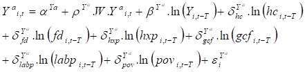 (27)
(27)
 (28)
(28)
where α:s,β:s, and δ:s are “parameters” to be assessed and “ε” is an “error term”. The hypothesis of spatial correlation relates to the parameter, P , where H0:ρ=0 is tested against the alternative, ρ,H1:ρ≠0. If H0 is rejected, we have two possibilities. First, a positive and significant result for projected r suggests a positive correlation between the agricultural development in neighboring countries, and that implies agricultural development in one country is bound to ‘spill over’ and have a positive effect on agricultural development rates in the neighboring countries. In addition, if the effect is negative, it shows that, depending on other explanatory variables, the development in one country has affects its neighbors adversely.
Spatial Error Model
For a spatial error model (SEM model), dependence among neighbouring regions will go through the error process because the errors from these regions may show spatial covariance. The variance between the spatial lag model stated in (27) and (28) and the spatial error model relate to ρ and the error term ε. ρ ≡ 0 and ε = λW+μ in the spatial error model. If we rearranging the above, ε=(I-λW)(-1) μ , where λ is the coefficient of scalar spatial error, μ~N(0,σ2 I) and the original error term has the non-spherical covariance matrix E[[εε’]=(I-λW)-1 σ2 I(I-λW)-1] . What this implies is that if the spatial error model is stated properly, not only will a random shock in one country will have effects on the country, but it will also spread to other regions as well.
In a model where there is presence of spatial lag and spatial error, it is not appropriate to use Ordinary Least Square (OLS) because of the problem of spherical disturbance. For example, in a spatial lag model, using Ordinary Least Square (OLS) generates subjective and unreliable evaluations. It will also bring about fair but ineffective parameter estimates and unreliable parameter variance in the spatial error model. As a result of this inconsistency, the Maximum Likelihood (ML), Instrumental Variable (IV) or Generalized Method of Moments (GMM) estimators have been recommended as alternatives to OLS (Anselin, 1988; Kelejian & Prucha, 1999). This therefore justifies our intention to verify the presence of spatial lag or spatial error in this article. If our tests for spatial lag and spatial error show the presence of either of the two or both, we can them employ either IV or GMM estimators as suggested by Anselin, (1988), and Kelejian & Prucha (1999).
METHODOLOGY, DATA MEASUREMENT AND SOURCES
To determine the effect of agricultural development on poverty level in Nigeria, we employ Fully Modified Ordinary Least Square (FMOLS) on the basis of Vector autoregressive (VAR) model results and the Canonical Cointegrating Regression (CCR) method. The Vector Autoregressive (VAR) model is commonly used to model multivariate time series. VAR model looks like the simultaneous equation model (SEM), but few and weak restrictions are imposed when specifying a VAR model (Sims, 1980 and Chowdhury, 1986). VAR proves to be a useful tool that can be used to analyze dynamic relationships among time series procedures because of its attractive characteristics. They are easy to estimate and they have good forecasting capabilities. In addition to this, researchers do not need to specify which variables are endogenous or exogenous since all variables are considered to be endogenous. VAR models consist of a set of relationships “that contain both the lagged values and the current values of all system variables” (Mcmillin, 1991 and Lu, 2001). The FMOLS is a non-parametric approach used to deal with serial correlation. It was designed originally by Philips and Hansen (1990) in order to give optimal estimates of cointegrating regressions. The method modifies Least Square in a bid to account for serial correlation effects and endogeneity in the regression. The CCR is closely related to the FMOLS, but instead uses stationary transformations of the data to get least square estimates in order to eliminate the long-run dependence between the cointegrating equation and stochastic regressors innovations.
To examine the neighbourhood effect on the relation between agricultural development and poverty level in Nigeria, we employ spatial econometrics which consist of the set of alternative approaches that can be used when dealing with spatial data samples (Anselin, 1988a). Spatial econometrics is a sub-field of econometrics which deals with spatial interaction (spatial autocorrelation) and spatial structure (spatial heterogeneity) in regression models. Models that integrated space or geography in the past were mostly found in special fields like “regional science, urban and real estate economics and economic geography” (Anselin, 1992a; Anselin and Florax, 1995a; Anselin and Rey, 1997; Pace et al, 1998). However, the use of spatial econometric methods has increased in several empirical investigations in more traditional areas of economics such as agricultural and environmental economics, labour economics, public economics, local public finance and demand analysis (Anselin and Bera, 1998; Anselin, 1999). Here, we focus on the spatial lag model (SAR model) and spatial error model (SEM model). The SAR model captures locational dependencies like external effects or spatial interactions. Growth in a particular region may increase as a result of growth in a neighbouring region. The effects of policies in one country could spread beyond the geographical boundaries of such a country and may affect the economic conditions of other neighbouring countries or regions. Not only this, if there is conflict (e.g. herdsmen conflicts, kidnappings, terrorism etc.) in countries at the border region, this could spread and hinder the economic condition of the neighbouring countries. The above then creates a need for spatial analysis of agricultural development and poverty reduction in this article. The spatial error model (SEM model) is usually applied when spatial autocorrelation occurs as a result of misspecification or inadequate delimitation of spatial units. When interactions among regions are not modelled, these interactions are restricted to the error terms.
Data Source
Annual secondary data between 1980 and 2020 were obtained from the publications of World Bank’s World Development Indicators (WDI) and the Worldwide Governance Indicators (WGI). Data on agricultural sector growth were proxied with (agricultural GDP per capita), non-agricultural sector (Total GDP minus Agricultural GDP). human capital, financial deepening, health expenditure, manufacturing and transportation, oil rent, control of corruption, government effectiveness and regulatory quality. Since poverty is multidimensional, we generate poverty index by computing Principal Components of human development indicators (i.e longevity, measured by life expectancy at birth which is intended to capture capability of leading a long and healthy life, rural development measured by per worker agricultural value added, real per capita income and consumption per capita which represents access to resources needed for a decent standard of living) (see Canudas-Romo, 2018; Mansi et al, 2020).
RESULTS AND DISCUSSIONS
To examine the effect of agricultural development on poverty level in Nigeria, we first examine the descriptive statistics of the variables used for the analysis. Our results show that the mean of agriculture growth, human capital, health expenditure, manufacturing, transportation, oil rent and poverty are on average around 5.622%, 3.873%, 1.228%, 29.014%, 35.514, 12.173% and 0.00% respectively, while financial deepening, control of corruption, government effectiveness and regulatory quality are on average -22.800%, -1.169%, -0.985% and -0.917% respectively. The deviations of this variables from their means are not large. This then suggests that these variables are good candidates for regression analysis. The results of summary statistics are presented in Table 1.
Table 1 Results of Descriptive Statistics of Variables (Log Values)
| Variable | N | Mean | SD | Median | Min | Max |
| pov | 40 | 0.00 | 1.66 | -0.89 | -1.56 | 2.88 |
| aggro | 40 | 5.62 | 8.87 | 3.93 | -4.38 | 55.58 |
| hc | 40 | 3.87 | 0.52 | 4.02 | 2.29 | 4.40 |
| findep | 40 | -22.80 | 0.72 | -22.74 | -23.91 | -21.29 |
| hexp | 40 | 1.23 | 0.13 | 1.16 | 0.91 | 1.62 |
| manuf | 40 | 29.01 | 0.28 | 28.91 | 28.70 | 29.53 |
| transp | 40 | 35.51 | 23.90 | 27.63 | 2.88 | 80.89 |
| oilrent | 40 | 12.17 | 6.13 | 11.72 | 1.51 | 26.43 |
| corpc | 40 | -1.17 | 0.09 | -1.19 | -1.43 | -0.89 |
| goveff | 40 | -0.99 | 0.09 | -0.95 | -1.22 | -0.89 |
| reguq | 40 | -0.92 | 0.14 | -0.97 | -1.35 | -0.66 |
After this, we examine the correlation among our variables. The results show no serious correlation among the variables used. Therefore, robustness of estimated coefficients of the regression model is ensured. These results are also presented in Table 2.
Table 2 Results of Correlation of the variables used
| Pov | aggro | Hc | Hexp | findep | manuf | transp | oilrent | corpc | goveff | reguq | |
| pov | 1.00 | ||||||||||
| aggro | -0.05 | 1.00 | |||||||||
| hc | 0.52 | 0.17 | 1.00 | ||||||||
| hexp | 0.39 | -0.28 | 0.31 | 1.00 | |||||||
| findep | -0.71 | -0.09 | -0.32 | -0.41 | 1.00 | ||||||
| manuf | 0.67 | -0.14 | -0.01 | 0.05 | -0.28 | 1.00 | |||||
| transp | 0.37 | -0.06 | -0.25 | 0.22 | -0.38 | 0.25 | 1.00 | ||||
| oilrent | -0.30 | -0.07 | -0.04 | 0.03 | 0.53 | -0.35 | -0.19 | 1.00 | |||
| corpc | 0.44 | -0.40 | 0.18 | 0.17 | -0.24 | 0.21 | 0.36 | -0.08 | 1.00 | ||
| goveff | -0.60 | -0.09 | -0.47 | -0.04 | 0.42 | -0.22 | -0.07 | 0.27 | -0.29 | 1.00 | |
| reguq | 0.51 | -0.33 | 0.22 | -0.08 | -0.28 | 0.26 | 0.35 | 0.05 | 0.58 | -0.37 | 1.00 |
To check if the data is stationary or not, we test for the unit root using General Least Square-Augmented Dickey Fuller (GLS-ADF) test (Elliot et al., 1996). This test has been shown to be better at testing for unit root (Elliot et al., 1996). The results are presented in Table 3.
Table 3
| Variables | Unit Root Test: Philip Perron Test
Level I(0) |
Unit Root Test: Philip Perron Test
FIRST DIFFERENCE I(1) |
Unit Root Test: General Least Square-Augmented Dickey Fuller
Test Level I(0) |
Unit Root Test: General Least Square-Augmented Dickey Fuller
Test FIRST DIFFERENCE I(1) |
| Pov | -1.414 | -5.533* | -1.041 | -1.067* |
| Aggro | -2.181 | -5.831* | -1.034 | -2.718* |
| Hc | -3.326 | -5.870* | 0.165 | 0.209* |
| Findep | -2.781 | -8.634* | -0.534 | -0.961* |
| Hexp | -3.983 | -9.139* | -2.192 | -3.535* |
| Manuf | -1.989 | -4.925* | -1.246 | -2.880* |
| Transp | -2.524 | -6.968 * | -1.605 | -2.930* |
| oilrent | -3.559 | -7.831* | -1.567 | -1.973* |
| Corpc | -2.989 | -6.223* | -2.484 | -3.275* |
| goveff | -4.948 | -10.148* | -1.533 | -2.739* |
| Reguq | -3.605 | -7.640* | -1.747 | -3.027* |
Source: Author’s calculation using STATA 14.
“*” depicts the stationarity of the series at 5% significance level.
Our results show that all our variables are stationary at first difference I(1). This justifies the use of the LRCOV since its use requires stationary at first difference. In order to ensure robust inference, we consider the potential heteroscedasticity and autocorrelation of unknown forms in the data. This brings about a need for the LRCOV matrix estimation. LRCOV has been widely applied to non-stationary time series analysis, such as the Philip-Perron unit root test (Phillips and Perron, 1988), Cointgration Tests (Marmol and Velasco, 2004) and Panel Cointegration Tests (Pedroni, 2004) and a model’s stability based on Fully Modified Ordinary Least Squares (FMOLS) (Hansen, 1992), Canonical Cointegrating Regression, with both I(1) and I(2) variables (Choi, Park and Yu, 1997), Fully Modified Value at Risk (FMVAR) and Fully Modified Generalized Method of Moments (GMM) estimation (Quintos, 1998). We take this into consideration by computing the covariance matrix in linear regression. The results are shown in Table 5.
Table 5 Long-Run Covariance of the variables used in the study
| Long Run Covariance: | |||||||||||
| VAR Pre-whitening = no | |||||||||||
| Kernel type = Bartlett | |||||||||||
| Bandwidth (Newey-West) = 2.3552 | |||||||||||
| Dof adjustment = 0 | |||||||||||
| Two-sided | D.pov | D.aggro | D.hc | D.findep | D.hexp | D.manuf | D.transp | D.oilrent | D.corpc | D.goveff | D.reguq |
| D.pov | .0773891 | .0074054 | -.0207312 | -.0726162 | -.0011128 | .0165732 | .0317131 | -.5115527 | -.0002869 | -.0002699 | .0021792 |
| D.aggro | .0074054 | .0052167 | -.0011418 | -.0043781 | .001449 | .0025626 | .0007885 | -.0283436 | -.0013417 | -1.96e-06 | -.0043845 |
| D.hc | -.0207312 | -.0011418 | .041079 | .0203443 | -.0010821 | -.0110578 | .0187079 | -.2334273 | -.001418 | -.0009205 | -.0052547 |
| D.findep | -.0726162 | -.0043781 | .0203443 | .1568797 | -.0045841 | -.0025315 | -.0119978 | 1.125943 | .0027114 | -.0021272 | .0007421 |
| D.hexp | -.0011128 | .001449 | -.0010821 | -.0045841 | .0089552 | -.0013196 | .0025679 | .0407446 | .000113 | .0016841 | -.0037185 |
| D.manuf | .0165732 | .0025626 | -.0110578 | -.0025315 | -.0013196 | .0166603 | .0040332 | -.0306126 | -.0022265 | .0003426 | -.0011481 |
| D.transp | .0317131 | .0007885 | .0187079 | -.0119978 | .0025679 | .0040332 | .2631834 | -.2125179 | .0098599 | .0019504 | .0172074 |
| D.oilrent | -.5115527 | -.0283436 | -.2334273 | 1.125943 | .0407446 | -.0306126 | -.2125179 | 30.28675 | .0100017 | .1068016 | .1864769 |
| D.corpc | -.0002869 | -.0013417 | -.001418 | .0027114 | .000113 | -.0022265 | .0098599 | .0100017 | .0052459 | -.0002067 | .0035951 |
| D.goveff | -.0002699 | -1.96e-06 | -.0009205 | -.0021272 | .0016841 | .0003426 | .0019504 | .1068016 | -.0002067 | .0038104 | .0004945 |
| D.reguq | .0021792 | -.0043845 | -.0052547 | .0007421 | -.0037185 | -.0011481 | .0172074 | .1864769 | .0035951 | .0004945 | .0137672 |
We select a lag length of 4 based on the results of Likelihood Ratio (LR), Akaike Information Criteria (AIC), Hanna Quine Information Criteria (HQIC) and Schwartz Bayesian Information Criteria (SBIC). The results are also presented in Table 6.
Table 6 Results of Lag Length of the variables used
| lag | LL | LR | df | p | FPE | AIC | HQIC | SBIC |
| 0 | -1295.11 | 9.0e+17 | 72.5615 | 72.7304 | 73.0454 | |||
| 1 | -1003.91 | 582.39 | 121 | 0.000 | 9.5e+13 | 63.1062 | 65.1328 | 68.9125 |
| 2 | -770.75 | 466.33 | 121 | 0.000 | 1.8e+12 | 56.875 | 60.7592 | 68.0036 |
| 3 | 5287.56 | 12117 | 121 | 0.000 | 7.e-125* | -272.975 | -267.234 | -256.524 |
| 4 | 10743.2 | 10911* | 121 | 0.000 | -574.842* | -568.762* | -557.423* |
Results and Discussions of the Effect of Agricultural Development on Poverty Level in Nigeria
To control for other factors that are associated with poverty, not linked to agriculture, as well as the potential nonlinearities of our explanatory variables, we use the natural logarithms of the regressors (Levine, Loazya and Beck, 2000).
Using the Fully Modified Ordinary Least Square (FMOLS), we find that 25% of the variation in poverty is explained by agriculture, human capital, financial deepening, health expenditure, manufacturing, transportation, oil rent, control of corruption, government effectiveness and regulatory quality. Our results show that agricultural growth, transportation, oil rent have a negative relationship with poverty. These results were statistically significant. However, human capital, financial deepening, health expenditure, manufacturing, transportation, oil rent, control of corruption, government effectiveness and regulatory quality do not reduce poverty and the results are statistically significant. Our results showed that, for every additional 10% increase in agricultural growth, the expected poverty level reduces by 0.389% on the average, holding all other variables constant. This gives credence to the hypothesis that the growth and development of the agricultural sector is capable of reducing the level of poverty in Nigeria.
As for human capital, for every additional 10% of human capital, the expected poverty level increases by 10.91% on the average, why 10% increase in financial development leads to increase in poverty level by 5.48% on the average. In the case of the health sector, for every additional 10% increase in health expenditure, poverty increased by 100.59%. For every additional 10% increase in the manufacturing sector, poverty level still increased by 19.87%. This could be as a result of government failure to provide necessary infrastructures in the economy. Most of the manufacturing industries prefer to operate in the neighbouring countries where there is availability of infrastructural facilities.
Control of corruption, government effectiveness and regulatory quality, which is used to represent the quality of institutions in Nigeria also failed to reduce poverty on their own, according to our FMOLS results. In essence, given our FMOLS results, only the agricultural sector, transportation and oil rent lead to a reduction in poverty and the results are statistically significant. These results are presented in Table 7.
Table 7 Results of the Effect of Agricultural Development on Poverty Level in Nigeria using FMOLS
| VAR lag(user) = 4 Number of obs = 39 | ||||||
| Kernel = qs R2 = .2454515 | ||||||
| Bandwidth(andrews) = 1.5836 Adjusted R2 = -.0240301 | ||||||
| S.e. = 1.680529 | ||||||
| Long run S.e. = 4.23e-14 | ||||||
| Pov | Coef. | Std. Err. | Z | P>|z| | [95% Conf. Interval] | |
| aggro | -.0388935 | 1.25e-15 | -3.1e+13 | 0.000 | -.0388935 | -.0388935 |
| hc | 1.090866 | 2.33e-14 | 4.7e+13 | 0.000 | 1.090866 | 1.090866 |
| findep | .5475143 | 2.32e-14 | 2.4e+13 | 0.000 | .5475143 | .5475143 |
| hexp | 10.05917 | 1.06e-13 | 9.5e+13 | 0.000 | 10.05917 | 10.05917 |
| manuf | 1.987262 | 3.53e-14 | 5.6e+13 | 0.000 | 1.987262 | 1.987262 |
| transp | -.0241085 | 5.13e-16 | -4.7e+13 | 0.000 | -.0241085 | -.0241085 |
| oilrent | -.1196354 | 1.61e-15 | -7.4e+13 | 0.000 | -.1196354 | -.1196354 |
| corpc | 1.927787 | 9.97e-14 | 1.9e+13 | 0.000 | 1.927787 | 1.927787 |
| goveff | .2049245 | 1.16e-13 | 1.8e+12 | 0.000 | .2049245 | .2049245 |
| reguq | 7.891094 | 9.16e-14 | 8.6e+13 | 0.000 | 7.891094 | 7.891094 |
| _cons | -49.59146 | 9.14e-13 | -5.4e+13 | 0.000 | -49.59146 | -49.59146 |
When we used the Canonical Cointegrating Regression (CCR), we also found that agricultural growth is expected to lead to a reduction in poverty, but generally, the results were slightly different. All the CCR results are also statistically significant. The CCR however shows a higher R-square. 97.475% of the variation in poverty is explained by agriculture, human capital, financial deepening, health expenditure, manufacturing, transportation, oil rent, control of corruption, government effectiveness and regulatory quality. It was discovered that a 10% increase in agricultural growth is expected to lead to a 0.124% reduction in poverty level. In other words, at the time of this study, for every additional 10% increase in agricultural growth, the expected poverty rate reduces by 0.124% on the average, holding all other variables constant. For every additional 10% increase in human capital, the expected poverty level increases by 13.18% on the average, holding all other variables constant. For every additional 10% increase in financial deepening, the expected poverty rate reduces by 16.43% on the average, holding all other variables constant. For every additional 10% increase in health expenditure, the expected poverty rate reduces by 10.15% on the average, holding all other variables constant. These results are presented in Table 7 and 8.
Generally, both the FMOLS and CCR results gives credence to the reasoning that developing agricultural sector can reduce the level of poverty in Nigeria. This corroborates the works of Cervantes-Godoy and Dewbre (2010), Azuh and Matthew (2010) and Oyakhilome and Zibah (2014).
Table 8. Results of the Effect of Agricultural Development on Poverty Level in Nigeria using Canonical Cointegrating regression (CCR)
| VAR lag(user) = 4 Number of obs = 39 | ||||||
| Kernel = qs R2 = .9747537 | ||||||
| Bandwidth(andrews) = 1.5836 Adjusted R2 = .9657372 | ||||||
| S.e. = .7847279 | ||||||
| Long run S.e. = 5.12e-15 | ||||||
| pov | Coef. | Std. Err. | Z | P>|z| | [95% Conf. Interval] | |
| aggro | -.0124308 | 6.31e-17 | -2.0e+14 | 0.000 | -.0124308 | -.0124308 |
| hc | 1.318491 | 1.12e-15 | 1.2e+15 | 0.000 | 1.318491 | 1.318491 |
| findep | -1.643249 | 1.11e-15 | -1.5e+15 | 0.000 | -1.643249 | -1.643249 |
| hexp | -1.015408 | 7.03e-15 | -1.4e+14 | 0.000 | -1.015408 | -1.015408 |
| manuf | 1.797264 | 3.61e-15 | 5.0e+14 | 0.000 | 1.797264 | 1.797264 |
| transp | .0026571 | 3.59e-17 | 7.4e+13 | 0.000 | .0026571 | .0026571 |
| oilrent | -.001829 | 9.55e-17 | -1.9e+13 | 0.000 | -.001829 | -.001829 |
| corpc | 3.761629 | 6.82e-15 | 5.5e+14 | 0.000 | 3.761629 | 3.761629 |
| goveff | -.4529917 | 8.54e-15 | -5.3e+13 | 0.000 | -.4529917 | -.4529917 |
| reguq | -.3374035 | 4.76e-15 | -7.1e+13 | 0.000 | -.3374035 | -.3374035 |
| _cons | -89.90307 | 9.23e-14 | -9.7e+14 | 0.000 | -89.90307 | -89.90307 |
Neighbourhood effect on agricultural development and poverty level in Nigeria between 1980 and 2019.
To determine the neighbourhood effect on agricultural development and poverty level in Nigeria between, we test for spatial autocorrelation in the residual as well as spatial lag, i.e. we try to check whether or not there is spatial autocorrelation on the error term models, with the use of Moran’s test statistics (Moran 1948, 1950a, 1950b). In a case where we regress the OLS model with data collected from all countries, the residual of the Ordinary Least Square model may be system positive in some countries and system negative in others, leading to the variance of the error term not being constant among different regions. When we have such a case, OLS would not be the best model to capture the relationship among the explanatory variable and the explained variables.
We build the spatial autoregression (SAR) model, with the use of a ‘spatial weight matrix’ (Wij) to measure the spatial correlation among different observations. In building a weight matrix, there is no rigid theoretical framework, but we can construct it according to the need of specific practice applications. However, one important rule is that the matrix should be exogeneous to the regression model (Manski, 1993).
For this study, we specified the components of the weight matrix as an inverse-distance matrix, with respect to the spatial distance between the observations or regions under study (Anselin, 1980). Region “i” could be our region (Nigeria), while region “j” is a neighbouring country (e.g. Niger). The spatial matrix shows the spatial relationship that exists between all the regions and the value of the elements is:
Wij= 1/(distance between i and j)
We get the distance between the regions i and j to be: ((lati-latj )2+(logj- logi)2)(1/2)
Where lati and logj represent the latitude and longitude of observations respectively.
Given how the matrix is built, when we have a higher value of the element Wij, it shows that the distance between i and j is shorter, while if Wij has a lower value, it shows that the distance between regions/observations i and j is larger.
To obtain a simpler form of this process, we can standardize the spatial weight matrix . A way of doing this is to divide each cell of matrix Wij by the summation of the respective row cells. Wij*=Wij/(∑(j=1)n Wij )
With this, we can generate the standard weighted matrix by using the equation above and the sum of each row equals 1. Given the standard weight matrix above, which shows the spatial structure of the observation, we can calculate the statistics of Moran’s I, with the following expression (Moran, 1948, 1950a, 1950b). I=(N/S0 )((e’We)/(ee’))
S0=∑i∑jWij
Where N represents “number of observations”, W is the “standardized weight matrix”, i and j are the “number of elements in the weight matrix” respectively, e represents the “residual of the regression model” and e’ represents the “transpose of e”. The “Moran’s I” statistics has a range of (-1, 1). The closer it is to -1, the more a dissimilar spatial structure is observed while the closer it is to 1, the more a similar spatial structure is observed. There are cases when the “Moran’s I” will be equal to 0. This indicates that there is no spatial autocorrelation problem. In order to get a more precise test, we can use the Z-scores and the hypothesis test (t-test) (Cliff & Ord, 1973, 1981). If the residuals of the OLS model are normally distributed, the “Moran’s I” would be distributed normally and we can use the Z-scores. A hypothesis test (t-test) can also be performed in such case to estimate whether the Moran’s I significantly differs from the value, which indicates no spatial autocorrelation.
The null hypothesis, H0 = There is no spatial autocorrelation (i.e., Moran’s I = 0). Alternative hypothesis, H1= There is spatial autocorrelation (Moran’s I ≠ 0). Here, the null hypothesis of Moran’s I test = 0, which indicates that there is no spatial autocorrelation. If the Z value is greater than 1.96, we would reject the hypothesis, then the spatial autocorrelation is significant at 95% confidence level.
Following the processes above, we first run diagnostic tests for spatial dependence in the OLS regression. The results of our Moran’s I and spatial lag weren’t significant. This means there is no significant spatial autocorrelation problem in the residual and no spatial lag problem in the model. The results of our diagnostic tests are presented in Table 10.
Table 10. Diagnostic tests for spatial dependence in OLS regression
| Type: Distance-based (inverse distance) | ||||
| Distance band: 0.0 < d <= 10.0 | ||||
| Row-standardized: Yes | ||||
| Diagnostics | ||||
| Test | Statistic | Df | p-value | |
| Spatial error: | ||||
| Moran’s I | 1.060 | 1 | 0.289 | |
| Lagrange multiplier | 0.199 | 1 | 0.655 | |
| Robust Lagrange multiplier | 0.099 | 1 | 0.753 | |
| Spatial lag: | ||||
| Lagrange multiplier | 0.126 | 1 | 0.722 | |
| Robust Lagrange multiplier | 0.026 | 1 | 0.871 | |
Our results corroborate that of previous studies such as Amao et al (2013), Oyakhilome and Zibah (2014), Adetayo (2014) and Margwa et al (2015), which concluded that agricultural development can indeed reduce poverty level in Nigeria. Also, our results show that there was no significant neighbourhood effect or spatial dependence. This therefore suggests that failure of agricultural development in reducing poverty level in Nigeria has no connection with her neighbouring countries.
CONCLUSION
In conclusion, this study provides insights into the role of agricultural development in reducing poverty level in Nigeria over a 39-year period (1980-2019). The study utilizes annual data and employs three statistical models: Fully Modified Ordinary Least Square (FMOLS), Canonical Cointegrating Regression (CCR), and spatial econometrics. The findings suggest that agricultural development can have a positive impact on poverty reduction in the country. The study also reveals that neighbouring countries did not have a significant influence on the relationship between agricultural development and poverty level in Nigeria. Based on the findings, the government should prioritize the improvement of agriculture, transportation, and oil rent, which can complement each other in reducing poverty in the country. The results of this study can inform policymakers and stakeholders on the need to enhance agricultural development as a key strategy for poverty reduction in Nigeria.
REFERENCES
- Adetayo, A. O. (2014). Analysis of farm households poverty status in Ogun states, Nigeria. Asian Economic and Financial Review, 4(3), 325-340.
- Amao, J. O., Ayantoye, K., & Fadahunsi, O. D. (2013). Poverty among farming households in Osun State, Nigeria. International Journal of Humanities and Social Science, 3(21), 135-143.
- Anfofum, A.A. and Olure-Bank, A.M. (2018). “Analysis of Oil Revenue and Economic Corrruption in Nigeria”. International and Public affairs; 2(1): 1-10
- Anselin, L., and S. Rey (1991). Properties of tests for spatial dependence in linear regression
- models. Geographical Analysis 23, 112–31.
- Anselin, L. (1992a). Space and applied econometrics. Special Issue, Regional Science and
- Urban Economics 22.
- Anselin, L. (1988a). Spatial Econometrics: Methods and Models. Kluwer Academic, Dordrecht.
- Anselin, L. (1988b). A test for spatial autocorrelation in seemingly unrelated regressions.
- Economics Letters 28, 335–41.
- Anselin, L., and R. Florax (1995a). Introduction. In L. Anselin and R. Florax (eds.) New
- Directions in Spatial Econometrics, pp. 3–18. Berlin: Springer-Verlag.
- Anselin, L., and R. Florax (1995b). Small sample properties of tests for spatial dependence
- in regression models: some further results. In L. Anselin and R. Florax (eds.) New
- Directions in Spatial Econometrics, pp. 21–74. Berlin: Springer-Verlag.
- Anselin, L., and S. Rey (1997). Introduction to the special issue on spatial econometrics.
- International Regional Science Review 20, 1–7.
- Anselin, L. (1988). Spatial Econometrics: Methods and Models Dordrecht: Kluwer Academic Publishers.
- Anselin, L. and Bera, J. (1998). “Spatial dependence in linear regression models with an introduction to spatial econometrics” in A. Ullah and D. Giles (eds) Handbook of Applied Economic Statistics New York: Marcel Dekker, pp. 237-289.
- Azuh, D. E., & Matthew, O. (2010). The role of agriculture in poverty alleviation and national development in Nigeria. African Journnal of Economy and Society, 10 (1&2), 17-32.
- Bigman, D and H.Fofack, (2000). Geographical Targeting for Poverty Alleviation: An Introduction to the Special Issue. The World Bank Economic Review
- Bourguignon, F., & Morrisson, C. (1990). Income distribution, development and foreign trade: A cross-sectional analysis∗. European economic review, 34(6), 1113-1132.
- Byerlee, D. de Janvry, A. and E. Sadoulet (2009), “Agriculture for Development: Toward a New Paradigm”, Annual Review of Resource Economics, Vol. 1: 15-35, October 2009.
- Canudas-Romo, V. (2018). Life expectancy and poverty. The Lancet Global Health, 6(8), e812-e813.
- Cervantes-Godoy, D. and J. Brooks (2008), “Smallholder Adjustment in Middle-Income Countries: Issues and Policy Responses”, OECD Food, Agriculture and Fisheries Working Papers, No. 12, OECD, Paris.
- Cervantes-Godoy, D. and J. Dewbre (2010), “Economic Importance of Agriculture for Poverty Reduction”, OECD Food, Agriculture and Fisheries Working Papers, No. 23, OECD Publishing. doi: 10.1787/5kmmv9s20944-en
- Choi, I., Park, J. Y., & Yu, B. (1997). Canonical cointegrating regression and testing for cointegration in the presence of I (1) and I (2) variables. Econometric Theory, 13(6), 850-876.
- Chowdhury, A.R. (1986). Vector Autoregression as Alternative Macro-modeling Technique:
- The Bangladesh Developement Studies, 14 (2), 21–32.
- Christiaensen, L. and L. Demery (2007), Down to Earth Agriculture and Poverty Reduction in Africa, The World Bank Group.
- Christiansen, L., Demery,L.&Kuhl, J. (2010). The role of agriculture in poverty reduction an empirical perspective. Journal of Development Economics. 3 – 7
- Cliff, A. D., & Ord, J. K. (1981). Spatial processes: models & applications. Taylor & Francis.
- Delgado, Christopher L., Jane Hopkins, and Valerie A. Kelly (1998): “Agricultural Growth
- Linkages in Sub-Saharan Africa”; IFPRI Research Report 107; International Food Policy
- Research Institute, Washington D.C.
- Diao, X. et al. (2010). The Role of Agriculture in African Development, World Development,
- doi:10.1016/j.worlddev.2009.06.011
- Elliot, G. (1996). Thomas J. rothenberg, and James H. Stock. Efficient Tests for an Autoregressive Unit root. Econometrica, 64(4), 813-836.
- FAO, 2006. Fao stat, fao, Nigeria, February, (2011). Available from: http//www.fao.org/faostat.
- Farrow, A ,Larrea, C., Hyman, G., Lema, G. (2005). Exploring the spatial variation of food poverty in Ecuador. Centro International de Agricultural Tropical (CIAT), AA67I3. Cali. Colombia
- Fields, G. S. (1980). Education and income distribution in developing countries: A review of the literature.
- Haggblade, Steven, Jeffrey Hammer, and Peter Hazell. 1991. “Modeling Agricultural Growth
- Multipliers”; American Journal of Agricultural Economics 73 (2): pp.361-374
- Hansen, B. E. (1992). Testing for parameter instability in linear models. Journal of policy Modeling, 14(4), 517-533.
- Henninger, N. (1998). Mapping and geographic analysis of human welfare and poverty: review and assessment. Washington, DC: World Resources Institute.
- Johnston, Bruce, and John Mellor, (1961), “The Role of Agricultural in Economic Development”,
- American Economic Review, No 4, pp. 566-93.
- Kelejian, H. H., & Prucha, I. R. (1999). A generalized moments estimator for the autoregressive parameter in a spatial model. International economic review, 40(2), 509-533.
- Lewis, William Arthur (1954): “Economic Development with Unlimited Supply of Labor”;
- Manchester School of Economic and Social Studies 22, May, 139-191.
- Levine, R., Loayza, N., & Beck, T. (2000). Financial intermediation and growth: Causality and causes. Journal of monetary Economics, 46(1), 31-77.
- Lipton, Michael (1977): Why Poor People Stay Poor: Urban Bias and World Development,
- Temple Smith, London, and Harvard University Press.
- Lu, M. (2001). Vector Autoregression (VAR) as Approach to Dynamic analysis of Geographic
- Processes. Geogr. Ann., 83 (2), 67–78. Poverty Reduct Ser. Retrieved from http://www.undp.orgpovertypublicationspovReview pdf
- Mansi, E., Hysa, E., Panait, M., & Voica, M. C. (2020). Poverty—A Challenge for Economic Development? Evidences from Western Balkan Countries and the European Union. Sustainability, 12(18), 7754.
- Manski, C. F. (1993). Identification problems in the social sciences. Sociological Methodology, 1-56.
- Margwa, R. S., Onu, J. I., Jalo, J. N., & Dire, B. (2015). Analysis of poverty level among rural households in Mubi region of Adamawa State, Nigeria. J. Sci. Res. Stud, 2(1), 29-35.
- Marmol, F., & Velasco, C. (2004). Consistent testing of cointegrating relationships. Econometrica, 72(6), 1809-1844.
- Mbam, B.N., &Nwibo S.U. (2013). Entrepreneurship Development as a Strategyfor Poverty Alleviation among farming Households in Igbo-Eze North LocalGovernment Area of Enugu State, Nigeria.Green Journal of Agriculturalscience. 3(10): 736 – 742.
- Mcmillin, W.D. (1991). The velocity of M1 in the 1980s: Evidence from a multivariate time
- series. Southern Economic Journal, 57 (3), 634–648.
- Mindy, S. Crandall, Bruce A. Weber (2004). Local Social and Economic Conditions, Spatial Concentrations of Poverty, and Poverty Dynamics. RPRC Working Paper No. 04-04
- Morris, C. T., & Adelman, I. (1988). Comparative patterns of economic development, 1850-1914. Johns Hopkins University Press.
- National Bureau of Statistics (NBS) (2020). “2020 Poverty and Inequality in Nigeria: Executive Summary”. National Bureau of Statistics Annual Reports.
- Ngbea, G.T. &Achunike, H.C. (2014). “Poverty in Northern Nigeria”. Asian Journal of Humanities and Social Studies. Vol. 2, No 2, ISSN:2321-2799.
- Ogbalubi, L.N. &Wokocha, C.C. (2013). Agricultural Development and Employment Generation: The Nigerian Experience. 10SR Journal of Agriculture and veterinary science. 2(2): 60 – 69
- Okwi, P..Ndeng’e, G., Kristjanson. P..Arunga, M.. Notenbaert, A., Omolo, A..Henninger, N., Benson. T .Kariuki, P. and Owuor. J. (2006). Geographic Determinants of Poverty in Rural Kenya: A National and Provincial Analysis. A Report prepared for the Rockefeller Foundation, Nairobi, Kenya.
- Olorunsanya, E. O., Falola, A., & Ogundeji, F. S. (2011). Comparative analysis of poverty status of rural and urban households in Kwara State, Nigeria.
- Oyakhilome, O. and Zibah, R. G. (2014) “Agricultural Production and Economic Growth in Nigeria: Implication for Rural Poverty Alleviation” in Quarterly Journal of International Agriculture 53 (2014), No. 3: 207-223
- Pace, R. K., Barry, R., & Sirmans, C. F. (1998). Spatial statistics and real estate. The Journal of Real Estate Finance and Economics, 17, 5-13.
- Pedroni, P. (2004). Panel cointegration: asymptotic and finite sample properties of pooled time series tests with an application to the PPP hypothesis. Econometric theory, 20(3), 597-625.
- Phillips, P. C., & Hansen, B. E. (1990). Statistical inference in instrumental variables regression with I (1) processes. The Review of Economic Studies, 57(1), 99-125.
- Phillips, P. C., & Perron, P. (1988). Testing for a unit root in time series regression. Biometrika, 75(2), 335-346.
- Quintos, C. E. (1998). Fully modified vector autoregressive inference in partially nonstationary models. Journal of the American Statistical Association, 93(442), 783-795.
- Ravallion, M. (1992). Poverty comparisons: a guide to concepts and methods. The World Bank.
- Ravallion, M., and G. Datt (1996): “How important to India’s Poor is the Sectoral Composition of
- Economic Growth?”;World Bank Economic Review 10(1), pp.1-25.
- Ravallion, M., and G. Datt (2002): “Why has Economic Growth been More Pro-Poor in Some
- States of India than Others?” Journal of Development Economics 65, pp. 381-400.
- Ramirez, M. T., &Loboguerrero, A. M. (2002). Spatial dependence and economic growth: Evidence from a panel of countries. Borradores de Economia Working Paper, (206).
- Ravallion, M., and S. Chen (2004): “China’s (Uneven) Progress Against Poverty” World Bank
- Policy Research Working Paper No. 3408.
- Schultz T. W. (1953). The Economic Organization of Agriculture (New York, 1953).
- Schultz T.W. (1964). Transforming Traditional Agriculture (New Haven, Conn., 1964). University Press.
- Sims, C.A. (1980). Macroeconomics and Reality. Econometrica, 48 (1), 1–48.
- Sowunmi, F., Akinyosoye, V., Okoruwa, V., &Omonona, B. (2012). The Landscape of Poverty in Nigeria: A Spatial Analysis Using Senatorial Districts-level Data. American Journal of Economics, 2(5), 61-74.
- Timmer, P. (1988), “The Agriculture Transformation”, Handbook of Development Economics,Vol. 1, Elsevier Science Publishers B.V.
- Townsend, R. (2015). Ending poverty and hunger by 2030: an agenda for the global food system (No. 95768, pp. 1-32). The World Bank.
- Umaru, A & Zubairu, A.A. (2012) An Empirical analysis of the contribution of agriculture and petroleum sector to the growth and development of the Nigerian economy from 1960- 2010, International Journal of Social Science & Education. Vol 2 (4). Available online
- Voss P.R, Long D.D., Roger B.H., Friedman S (2006)., “County Child Poverty Rates in the US: A Spatial Regression Approach”, Popul Res Policy Rev, no. 25, pp. 369–391
- World Bank (2000): The Quality of Growth, Oxford University Press: Oxford.
- World Poverty Clock https://www.worldpoverty.io/headline/