
On the Banking Deepening and Economic Volatility Nexus in Emerging Countries: Evidence from a GMM Panel-VAR Approach
- Meriem Sebai
- Omar Talbi
- Hella Guerchi Mehri
- 430-442
- May 30, 2024
- Economics
On the Banking Deepening and Economic Volatility Nexus in Emerging Countries: Evidence from a GMM Panel-VAR Approach
Meriem Sebai, Omar Talbi, Hella Guerchi Mehri
University of Tunis El-Manar, TUNISIA
DOI: https://dx.doi.org/10.47772/IJRISS.2024.805032
Received: 10 April 2024; Revised: 26 April 2024; Accepted: 30 April 2024 Published: 30 May 2024
ABSTRACT
This study investigates the dynamic causal relationship between banking deepening and economic growth volatility in 38 emerging countries from 1985 to 2020.To accomplish this, a panel autoregressive vector within a generalized method of moments framework is employed.Furthermore, impulse response functions are utilized to scrutinize the reaction of banking deepening aftershocks on economic volatility and vice versa. Finally, the analysis extends to include forecast error variance decompositions of the variables. The results underscore compelling evidence indicating that positive shocks in banking deepening significantly contribute to heightened economic volatility. Conversely, nations characterized by elevated economic volatility tend to exhibit restrained progress in banking deepening. These findings emphasize the urgent need for policymakers to implement stronger financial regulatory measures, bolstering risk management protocols and oversight mechanisms.
Keywords: Banking deepening, Economic growth volatility, Panel vector auto-regression, Impulse-response function, Emerging countries.
INTRODUCTION
Financial development, epitomized by the expansion and reinforcement of financial systems, has profoundly shaped global economies. Particularly during 1980-1990, a pronounced wave of financial development surged across nations, especially in emerging economies. This transformative process led to the establishment of robust financial institutions and an enhancement of banking services, ultimately deepening the financial sector. This yielded striking advancements in credit accessibility and the expansion of financial mediation, catalyzing overall economic growth and prosperity. Diverse scholars, notably (King and Levine (1993), Levine (1997), Rajan and Zingales (1998)) comprehensively affirm the merits of an enhanced financial system, thereby solidifying the beneficial link between financial development and economic growth. Nonetheless, economic volatility induces capricious oscillations that can reverberate through markets and economies (Ibrahim and Alagidede (2017)). This phenomenon has garnered significant interest among economists and policymakers, given the imperative to comprehend the interaction between financial development and economic volatility. This understanding is pivotal for ensuring the sustainable development of the economy.
The exploration of theoretical studies focusing on the relationship between financial development and economic volatility has led to the emergence of three distinct paradigms. The first paradigm, put forth by (Bernanke and Gertler (1989), Kiyotaki and Moore (1997), Aghion et al. (1999)), posits that a mature financial system plays a vital role in alleviating economic volatility. According to this perspective, a robust financial system helps to attenuate economic volatility by mitigating financial constraints, facilitating smoother credit flow, and enhancing risk management mechanisms. On the other hand, Greenwald and Stiglitz (1991), Mishkin (1996), Acemoglu and Zilibotti (1997), Bacchetta and Caminal (2000), Aghion et al. (2004), Morgan et al. (2004), and Shleifer and Vishny (2010) propose a more nuanced perspective. This view suggests that the relationship between financial development and economic instability is multifaceted, contingent on several factors, such as the level of financial development, the impacts of both real and monetary shocks, and the potential for diversification within the financial sector. Nevertheless, by introducing a theoretical model, López-Monti (2020) elucidates an alternative perspective on the causal relationship between financial deepening and economic volatility.
In the empirical landscape, extensive research has delved into the impact of the financial sector’s depth on economic volatility. Previous studies by Da-Silva (2000), Raddatz (2006), Manganelli and Popov (2015),Tang and Abosedra (2020), Kapingura, Mkosana and Kusairi (2022), Abanikanda and Dada (2023),Singh, Abosedra, Fakih, Ghosh and Kanjilal (2023), Song, Gong and Song (2024)emphasize the positive effect of a well- developed financial system. Such a system can reduce agency costs and improve credit market imperfections by efficiently gathering information on debtors. A different viewpoint has emerged from the works of Arcand, Berkes, and Panizza (2012), Ibrahim, and Alagidede (2017), Ma and Song (2017), Xue (2020), Ghosh and Adhikary (2023). These scholars indicate a U-shaped relationship between financial development and economic instability, suggesting that while initial financial development decreases economic volatility, this effect may reverse beyond a certain threshold. Kunieda (2008) further investigates this association, uncovering a concave pattern. Additional investigations conducted by Zouaoui, Mazioud, and Ellouz (2018) revealing an S-shaped relationship between banking deepening and economic growth volatility, characterized by multiple turning points.Furthermore, the intricate relationship between financial development and economic volatility is compounded by various influencing determinants. Some researchers emphasize the crucial role played by the quality of institutions, where the impact can vary significantly (Acemoglu et al., 2003, Struthmann et al., 2023). Additionally, economic, monetary, and real shocks have been identified as significant variables shaping this link (Denizer et al., 2002; Mallick, 2014; Ibrahim and Alagidede, 2017; Xue, 2020). Moreover, Alimi and Aflouk (2016) report a positive impact of real shock on economic volatility in developing and emerging countries.
Based on the discussion above, the lack of clarity surrounding the empirical relationship between financial deepening and economic volatility presents challenges for establishing a consensus on its direction. One plausible explanation for this ambiguity is the limited consideration given to the dynamic nature of this relationship and the potential for reverse causality. By examining the existing literature, evidence emerges suggesting a causal influence between banking deepening and economic growth volatility. Consequently, attempts to explain the association between these two variables using a single equation may lead to misleading results. The analysis aims to ascertain both effects: the impact of banking deepening on economic volatility and the impact of economic volatility on banking deepening. To accomplish this, panel vector autoregression (PVAR) model is employed within a generalized method of moments (GMM) framework, alongside the estimation of impulse response functions (IRFs).To the best of our knowledge, there is no study employing this method in this specific context.
Specifically, this study focuses on a sample of 38 emerging countries covering the period from 1985 to 2020. Exploring this link within emerging countries contributes significantly to the literature. Emerging economies exhibit discernibly less robust banking supervision, credit misallocation and more persistent output volatility compared to developed nations. The presence of limited technological infrastructure and production impediments might potentially encumber financial sector operations (Lopèz-Monti (2020), Barik and Pradhan (2021)). This study provides new evidence of a dynamic causal link between banking deepening and economic instability.
The paper’s structure is as follows: Section 2 discusses the sample and variable definitions. Section 3 outlines the panel VAR methodology. Section 4 presents empirical results. Section 5 concludes by summarizing findings and implications.
DATA DESCRIPTION, VARIABLES AND DESCRIPTIVE STATISTICS
Data
This research aims to examine the dynamic interrelationship between banking deepening and economic growth volatility. Using data from the World Bank’s World Development Indicators (WDI), a sample of 38 emerging countries[1] from 1985-2020 is employed. Table 1 provides descriptive statistics, offering an overview of key variables across the complete sample.
Variables measures and descriptive statistics
Measure of banking deepening (D_Credit):
Building on previous research conducted by Ibrahim and Alagidede (2017), Zouaoui and al. (2018), this study employs the domestic credit to private sector (% of GDP) as a widely acknowledged proxy for measuring banking system depth.
Measure of economic growth volatility (Eco_Vol):
As an indicator of economic growth volatility, the standard deviation of the GDP growth rate over a five-year period[2] is adopted, in line with Ma and Song (2017).
Table 1. Descriptive statistics of the main variables.
| Variables | Obs | Mean | Standard
Deviation |
Min | Max | Q1 | Q3 |
| D_Credit | 1165 | 0.3903 | 0.2848 | 0 | 1.5851 | 0.1919 | 0.5079 |
| Eco_Vol | 1299 | 0.0297 | 0.0317 | 0.0011 | 0.4878 | 0.0137 | 0.0358 |
Note. The analysis delineates that the average economic volatility (Eco_Vol) stands at 2.97%, with a range spanning from 0.11% to 48.78%. Similarly, the banking deepening (D_Credit) variable exhibits a positive mean of 39.03%, characterized by a relatively higher volatility level at 28.48%.
THE PANEL VAR METHODOLOGY:
Based on the study of Monti-Lopèz (2020) suggesting a causality realized relationship between banking deepening and economic growth volatility, this paper aims to evaluate this dynamic interrelationship using the Panel Vector Auto-Regression (P-VAR) approach. The VAR approach, originally introduced by Holtz-Eakin et al. (1988) and later refined by Sims (1980) for panel data analysis, is widely regarded as the most appropriate in the literature for several reasons. Firstly, it treats all variables in the model as endogenous simultaneously, capturing the endogenous interactions between banking deepening and economic volatility (Abbrigo and Love (2016)). Secondly, the P-VAR approach leverages cross-sectional data and allows for the inclusion of unobserved individual heterogeneity as fixed effects (Zouaoui and Zoghlami (2020)). These features enable a comprehensive understanding of the complex interplay between banking deepening and economic growth volatility.
According to the literature, the PVAR model is described as follows:
Zit = W0 + W(K)Zi,t + gi + εi,t, i = (1…N),t = (1985…2020) 1
Where
Zit : This vector encompasses the dependent variables measuring banking deepening (D_Credit) and economic growth volatility index (Eco_Vol). W0 : is a vector of constants. ![]() : represents a matrix polynomial of delayed coefficients. gi : controlling for fixed effects to account for the influence of the lagged dependence variable. εit : is a vector of idiosyncratic errors such as countries estimation errors.
: represents a matrix polynomial of delayed coefficients. gi : controlling for fixed effects to account for the influence of the lagged dependence variable. εit : is a vector of idiosyncratic errors such as countries estimation errors.
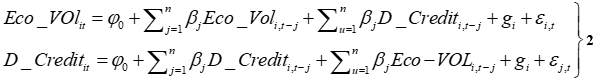
By adopting this regression for the main variables, i.e. banking deepening and economic instability, the models can be rewritten as follows:
Banking Deepening (D_Credit) and Economic growth volatility (Eco_Vol) Model:
EMPIRICAL RESULTS
The utilization of the panel VAR method requires the presence of a stationary distribution over time among the variables of interest. Furthermore, the determination of the lag order (p) in the panel specification is necessary to conduct Granger’s causality test. This choice is important as it influences the model’s structure and can significantly affect the test results. Subsequently, an analysis of the stability of the model (P-VAR) is presented, affirming its reliability and robustness. The findings of the panel VAR model are then outlined, providing insights into the dynamic relationships between the variables of interest. Moreover, the results of the estimation of the response function to the impulse are provided, shedding light on the short-term dynamics of the system. Finally, the decompositions of the forecasting error variance (FEVD) are detailed, helping to understand the relative importance of each variable in explaining forecast errors.
Panel unit root test
To apply the P-VAR model, assessing variable stationarity is crucial, as emphasized by Hartwig (2010). The Fisher-type unit root test, including Dickey-Fuller (ADF), Philips-Perron (PP) tests, and Im, Pesaran, and Shin (2003) test (IPS), is employed. The outcomes of the panel unit root test are presented in Table 2. The findings indicate the null hypothesis of unit root in all panels for Eco_Vol and D_Credit at the level cannot be rejected. However, results demonstrate these variables attain stationarity in first difference, supporting their suitability for P-VAR analysis.
Table 2. Unit root test
| Tests | Levels | First difference | ||
| D_Credit | Eco_Vol | D_Credit | Eco_Vol | |
| ADF | 2.7763 | -3.2827*** | -12.9115*** | -13.9852*** |
| PP | 4.1004 | -2.8168*** | -20.1955*** | -26.5034*** |
| IPS | 2.5805 | -2.8475*** | -11.6685*** | -12.7743*** |
Note.***indicates 1% significance. Max lags = one.
Panel VAR lag selection
Table 3 presents panel VAR models for interest variables. The preferred model follows Andrews and Lu’s (2001) criteria, favoring the first-order panel VAR due to lower MBIC, AIC, and MQIC values.
Table 3. PVAR Lag-Selection Criteria
| Lag | CD | MBIC | MAIC | MQIC |
| Model:
D_Credit and Eco_Vol 1 2 3 4 |
0.9913224
0.9900536 0.9909481 0.9781355 |
-205.7356
-184.0993 -159.9879 -142.2572 |
-32.92946
-30.4939 -25.58316 -27.05313 |
-98.94969
-89.17855 -76.93223 -71.06662 |
Note. CD, MBIC, MAIC and MQIC represent the global determination coefficients, the Bayesian information criteria, the Akaike information criterion and the Hannan-Quinn information criterion, respectively, based on criteria for selecting moments and coherent models.
Stability of the panel VAR model:
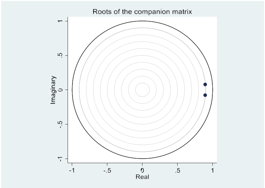
To assess the stability of the panel VAR model estimation, it is necessary to examine its stability condition. A reliable method for determining the stability of the panel VAR is to compute the modulus of each eigenvalue associated with the model (Lutkepohl, 2005). The eigenvalues of the P-VAR model (Eq. 2) are reported in Table 4, demonstrating that the magnitude of each eigenvalue is strictly below one, thus satisfying the stability condition. Furthermore, Figure. 1 confirms the stability of the estimated P-VAR model by illustrating that all eigenvalues lie within the unit circle.
Table 4. Eigen value stability condition
| Model | Eigenvalue | Modulus | |
| Real | Imaginary | ||
| Model:
D_Credit andEco_Vol |
0.8926711
0.8926711 |
-0.0777529
-0.0777529 |
0.8960509
0.8960509 |
Figure. 1. Graphic of the stability condition of Eigen value
Granger causality tests and panel VAR estimations
The P-VAR model treats all study variables as endogenous. Hence, prior to P-VAR estimation, it is imperative to scrutinize reverse causality within interest variables. The presence of reverse causality is signaled by p-values below 5% (see table 5).
Table 5. Granger-causality test
| Model | Null Hypothesis | Chi² | P-value |
| Model:
Banking deepening (D_Credit) and economic volatility (Eco_Vol) |
D_Credit (excluded) does not granger cause Eco_Vol
Eco_Vol (excluded) does not granger cause D_Credit |
38.898***
20.912*** |
0.000
0.000 |
Note. ***denotes statistical significance at the 1% level.
Table 6 below presents the results of the P-VAR estimation using a GMM model, as shown in equation (2). The findings consistently affirm that expanding banking deepening (D_Creditt-1) corresponds to heightened economic growth volatility across all specifications, aligning with prior studies, such as Zouaoui et al. (2018). These earlier researches emphasize the positive impact of banking deepening on economic volatility, especially in its potential to destabilize emerging economies by increasing domestic credit to the private sector as a percentage of GDP. This results in an inefficient credit distribution within the economy, which can impede risk-sharing mechanisms and lead to credit misallocation, potentially contributing to economic instability.
Turning the focus to the impact of economic volatility on banking deepening, a robust and statistically significant negative effect of economic growth volatility on banking deepening is observed across all specifications. These findings further bolster the argument posited by Lopèz-Monti (2020), suggesting that a nation grappling with intrinsic volatility in the real sector could result in an underdeveloped financial system as a byproduct of this instability.
Table 6. Estimation results of the panel-VAR models: D_Credit and Eco_Vol
| Variables | Reg (1) :
Eco_Vol |
Reg :
D_Credit |
Reg (2) :
Eco_Vol |
Reg:
D_Credit |
Reg (3) :
Eco_Vol |
Reg :
D_Credit |
Reg(4) :
Eco_Vol |
Reg :
D_Credit |
Reg (5) :
Eco_Vol |
Reg:
D_Credit |
| 0.041***
(0.000) |
1.023***
(0.000) |
0.039***
(0.000) |
1.014***
(0.000) |
0.034***
(0.000) |
1.028***
(0.000) |
0.032***
(0.000) |
1.039***
(0.000) |
0.033***
(0.000) |
1.034***
(0.000) |
|
| 0.763***
(0.000) |
-0.573***
(0.000) |
0.754***
(0.000) |
-0.575 ***
(0.000) |
0.885 ***
(0.000) |
-1.292***
(0.000) |
0.930***
(0.000) |
-1.649***
(0.000) |
0.949***
(0.000) |
-1.412***
(0.000) |
|
| Hansen’s test (p-value) | 0.138 | 0.241 | 0.392 | 0.316 | 0.220 | |||||
| N.Obs | 1034 | 1034 | 1034 | 1034 | 1034 |
Note. ***, ** and * indicate statistical significance at 1%, 5% and 10% levels, respectively.
Impulse response function (IRFs)
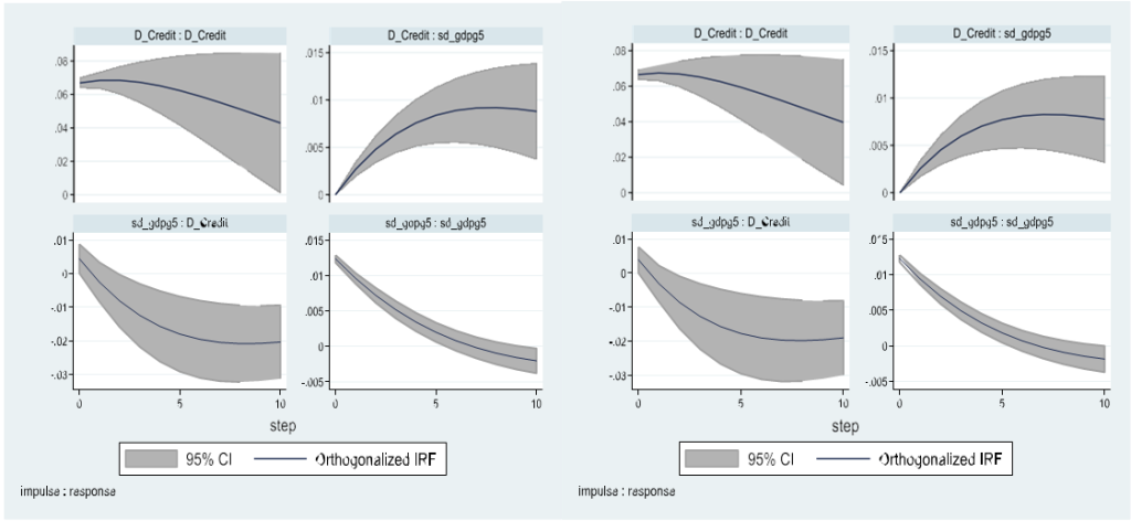
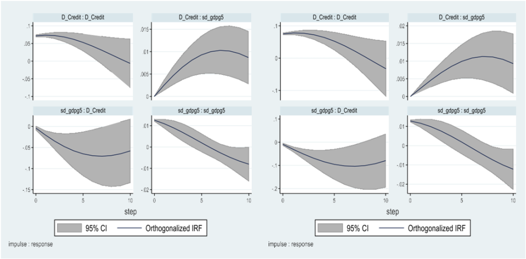
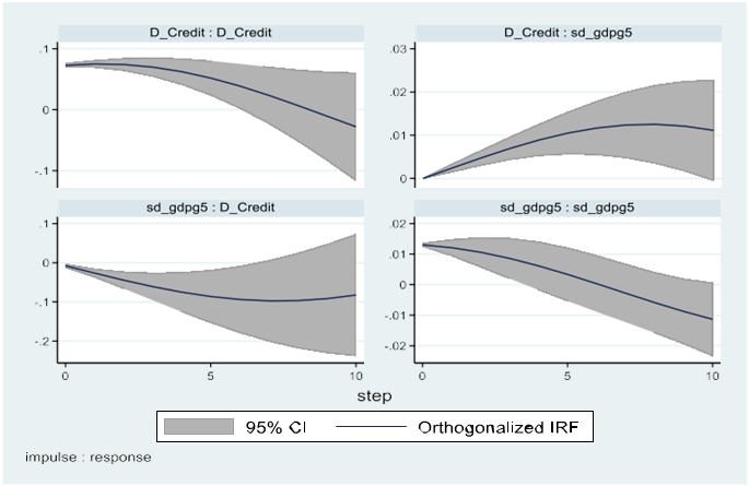
This function serves as a valuable tool for demonstrating the evolution of the variables of interest over a specific time horizon following a shock at a particular moment. Figure 2 displays the graphs depicting the impulse response functions (IRFs) that correspond to the specifications outlined in Table 6.
Based on the observations evident in Figure 2, a conspicuous pattern emerges wherein the graphs representing banking deepening (D_Credit) consistently maintain a positioning above the zero line. This consistent placement serves to underscore a discernibly positive responsiveness of banking deepening to perturbations in economic growth volatility (Eco_Vol). Notably, this favorable effect exhibits a progressive strengthening from period 0 to period 5.For instance, a shock of one standard deviation in banking deepening results in an increase in economic volatility of approximately 0.003 by the second year and around 0.008 by the tenth year.Conversely, the graphical depictions illustrating the reaction of banking deepening to the shocks in economic volatility demonstrate a diminishing trend across periods zero to five. Nevertheless, it is imperative toemphasize that this decline persists, thus suggesting a sustained influence on banking deepening. In light of these observations, a novel vantage point emerges, shed light on the dynamic interrelationship between banking deepening and economic growth volatility.
Figure. 2. Impulse-response function plots corresponding to the specifications in Table 6.
(1) (2)
(3) (4)
(5)
The forecast error variance decomposition (FEVD)
The impulse response function is analyzed by determining the variance decompositions of prediction error (FEVD). This process relies on the Cholesky decomposition of the residual covariance matrix derived from the estimated P-VAR model. The proportions of FEVDs for a 10-year forecast horizon are presented in Table 7.
Primarily, it is noteworthy that economic growth volatility (Eco_Vol) accounts for up to 64.85% of the variation observed in banking deepening. This indicates that changes in economic conditions, such as prolonged periods of economic instability or growth, can have enduring impacts on the deepening of the banking sector, leading to lasting changes in its structure and activities. In contrast, it is also significant to note that banking deepening (D_Credit) can explain as much as 56.16% of the variation in economic growth volatility. Over the long term, changes in the depth of banking activities, such as credit expansion or contraction, can have far-reaching consequences for economic stability and volatility.
Table 7. Forecast-error variance decomposition
| Model: D_Credit/Eco_Vol | ||
| ResponseVariable and horizon | impulsevariable | |
| Eco_Vol | D_Credit | |
| Eco_Vol | ||
| 0 | 0 | 0 |
| 1 | 1 | 0 |
| 2 | 0.982149 | 0.0178511 |
| 3 | 0.9380376 | 0.0619625 |
| 4 | 0.8676317 | 0.1323683 |
| 5 | 0.7760243 | 0.2239757 |
| 6 | 0.6743709 | 0.3256291 |
| 7 | 0.5780022 | 0.4219978 |
| 8 | 0.5016776 | 0.4983225 |
| 9 | 0.4545949 | 0.545405 |
| 10 | 0.4383126 | 0.5616874 |
| D_Credit | ||
| 0 | 0 | 0 |
| 1 | 0.0113403 | 0.9886597 |
| 2 | 0.065068 | 0.934932 |
| 3 | 0.1426719 | 0.8573281 |
| 4 | 0.2320232 | 0.7679768 |
| 5 | 0.3237849 | 0.676215 |
| 6 | 0.4114164 | 0.5885836 |
| 7 | 0.4904691 | 0.5095308 |
| 8 | 0.557821 | 0.4421791 |
| 9 | 0.6111171 | 0.3888829 |
| 10 | 0.6485038 | 0.3514962 |
Robustness test
In the subsequent analysis, a robustness assessment is conducted to examine the sensitivity of the initial findings. To achieve this, the panel VAR model presented in equation (2) is estimated, utilizing alternative indicators of banking deepening. These alternative measures were collected over a study period spanning from 1990 to 2020[3].
Table 8. Panel VA Rusing alternative measures of banking deepening
| Eco_Vol/Deposit_Bank | Eco_Vol/Lquid_Liab | |||
| Regressand:
Eco_Vol |
Regressand:
Deposit_Bank |
Regressand:
Eco_Vol |
Regressand:
Liquid_Liab |
|
| 𝐄𝐜𝐨_𝐕𝐨𝐥𝐭−𝟏 | 0.539***
(0.000) |
-1.164***
(0.000) |
0.728
(0.000) |
-0.607***
(0.006) |
| 𝐃𝐞𝐩𝐨𝐬𝐢𝐭_𝐁𝐚𝐧𝐤𝐭−𝟏 | 0.162***
(0.000) |
0.997***
(0.000) |
||
| 𝐋𝐢𝐪𝐮𝐢𝐝_𝐋𝐢𝐚𝐛𝐭−𝟏 | 0.139***
(0.000) |
0.968***
(0.000) |
||
| Numberofobs. | 208 | 208 | ||
| Eigenvaluestability
Condition |
0.852 | 0.888 | ||
| Granger-Causality
Waldtest |
0.000 | 0.000 | ||
Note. ***, ** and * indicate statistical significance at 1%, 5% and 10% levels, respectively. The p-values are shown in parentheses. Deposit_Bank: deposit money bank assets as a percentage of GDP. Liquid_Liab: Liquid liabilities to GDP. Eco_Vol: standard deviation of GDP growth.
CONCLUSION
This paper explores the dynamic interrelationship between banking deepening and economic growth volatility across 38 emerging countries from 1985 to 2020. To fulfill this goal, panel vector autoregression (P-VAR) models are employed within a generalized method of moments (GMM) framework, complemented by the application of impulse response functions (IRFs). This research adopts an innovative approach that considers all variables within the model as endogenous. Our findings disclose a positive effect of banking deepening on economic instability. This observation aligns with the conclusions drawn by Chen (2023).The positive coefficient attributed to banking deepening is underpinned by the excessive domestic credit to the private sector (% of GDP) and inadequate supervisory oversight. Conversely, heightened economic volatility fosters a climate of increased risk aversion among investors and lenders. This prompts a more cautious lending approach and restricts access to essential banking services for both enterprises and households. Consequently, the adept management of economic volatility emerges as a pivotal consideration for financial institutions, necessary to ensure a resilient and robust trajectory for banking deepening. Notably, these results demonstrate robustness when considering alternative measures of banking deepening.
The implications of our findings carry substantial weight for financial regulators and overseers in emerging economies. These nations face a multitude of challenges, and this research provides a valuable roadmap for addressing these issues. Policymakers in emerging economies are strongly encouraged to carefully calibrate the degree of banking deepening, while closely monitoring its trajectory to foresee and mitigate potential risks of economic imbalance. Encouraging banks to diversify their sources of funding beyond traditional deposits can also reduce their vulnerability to economic shocks and alleviate the risk of recessions. Moreover, regulators must actively promote the adoption of robust risk management practices within financial institutions, while ensuring diversified credit allocation across multiple segments. This strategic approach is designed to mitigate the concentration of risk within a single sector, thereby pre empting potential hazards. By adhering to these recommendations, financial regulators in emerging economies can adeptly manage the challenges associated with the deepening of the banking sector and economic instability, consequently fostering the sustainable development of the economy. Overall, this paper offers new insights into the dynamic interrelationship between banking deepening and economic growth volatility.
REFERENCES
- Abanikanda, E.O., Dada, J.T. (2023). External shocks and macroeconomic volatility in Nigeria: does financial development moderate the effect?. PSU Research Review.
- Abrigo, M.R.M., Love, I. (2016). Estimation of panel vector autoregression in Stata. Stata J. Prom. Commun. Stat. Stata, Vol. 16(3),pp. 778–804. https://doi.org/10.1177/1536867×1601600314.
- Acemoglu, D., Zilibotti, F. (1997). Was Prometheus Unbound by Chance? Risk, Diversification, and Growth. Journal of Political Economy, Vol. 105, pp. 709-751.
- Acemoglu, D., Johnson, S., Robinson, J., Thaicharoen, Y. (2003). Institutional causes, macroeconomic symptoms: Volatility, crises and growth. Journal of Monetary Economics, Vol. 50(1), pp. 49-123.
- Aghion, Ph., Banerjee, A., Piketty, T.H., (1999). Dualism and Macroeconomic Volatility. Quarterly Journal of Economics, Vol. 114(4), pp. 1359-1397.
- Aghion, Ph., Angeletos, G.M., Banerjee, A., Manova, k. (2004). Volatility and Growth: Financial Development and the Cyclical Composition of Investment. Journal of Monetary Economics, Vol. 51, pp. 1077–1106.
- Alimi, N., Aflouk, N. (2016). Terms-of-trade shocks and macroeconomic volatility in developing countries: panel smooth transition regression models. The Journal of International Trade & Economic Development, DOI: 10.1080/09638199.2016.1278029.
- Bacchetta, Ph., Caminal, R. (2000). Do capital market imperfections exacerbate output fluctuations? European Economic Review, Vol. 44, pp. 449-468.
- Barik, R., Pradhan, A.K. (2021). Does financial inclusion affect financial stability: Evidence from BRICS nations? The Journal of Developing Areas, Vol. 55(1), pp. 342-356.
- Bernanke, B., Gertler, M. (1989). Agency Costs, Net Worth, and Business Fluctuations. The American Economic Review, Vol. 79, pp. 14-31.
- Chen, W. (2023). The Effect of Financial Development on Economic Growth and Economic Volatility. BCP Business & Management, Vol. 38, pp. 717-734.
- Da-Silva, G. F. (2000). The impact of financial system development on business cycles volatility: Cross-country evidence. Journal of Macroeconomics, Vol. 24(2), pp. 233-253.
- Gosh, P., Adhikary, M. (2023). Dynamicity and nonlinearity in the association between different facets of financial development and macroeconomic volatility: evidence from the World Economy. International Review of Applied Economics, Vol. 37(6).
- Greenwald, B., Stiglitz, J. (1991). Financial Market Imperfections and Business Cycles, Quarterly Journal of Economics, Vol. 108, pp. 77-114.
- Hartwig, J. (2010). Is health capital formation good for long-term economic growth? – Panel Granger-causality evidence for OECD countries. J. Macroecon, Vol. 32 (1), pp. 314–325.
- Holtz-Eakin, D., Newey, W., Rosen, H. (1988). Estimating vector autoregressions with panel data. Econometrica, Vol. 56 (6), pp. 1371–1395. https://doi.org/10.2307/1913103.
- Ibrahim, M., Alagidede, P. (2017). Financial sector development, economic volatility and shocks in sub-Saharan Africa. Physica A: Statistical Mechanics and its applications, Vol.484, pp. 66– 81.
- Kapingura, F.M., Mkosana, N., Kusairi, S. (2022). Financial sector development andmacroeconomic volatility: Case of the SouthernAfrican Development Community region. Cogent Economics & Finance, Vol. 10(1), pp. 1-17.
- King, R., Levine, R. (1993a). Finance and growth: Schumpeter might be right. The Quarterly Journal Of Economics, Vol. 108(3), pp. 717-737. Available at: https://doi.org/10.2307/2118406.
- Kiyotaki, N., Moore, J., (1997). Credit Cycles. Journal of Political Economy, Vol. 105(2), pp. 211-248.
- Kunieda, T. (2008). Financial Development and Volatility of Growth Rates: New Evidence. Ryukoku University mimeo. Available at https://mpra.ub.unimuenchen.de/11341/1/MPRA_paper_11341.pdf
- Levine, R. (1997). Financial development and economic growth: Views and agenda. Journal of Economic Literature, Vol. 35(2), pp. 688-726.
- Lopèz-Monti, M. (2020). The Effect of Macroeconomic Volatility on Financial Deepening: A Missing Link?. Available at: https://www.rafalopezmonti.com/uploads/1/2/2/6/122625603/macro_volatility_and_financial _deepening_rafael_lopez-monti_nov_2020.pdf.
- Lutkepohl, H. (2005). New introduction to Multiple Time Series Analysis. Springer, New York.
- Ma, Y., Song, K. (2017). Financial Development and Macroeconomic Volatility. Bulletin of Economic Research, Vol. 70(3), pp. 205-225.
- Mallick, D. (2014). Financial development, shocks, and growth volatility. Macroeconomic Dynamics, Vol. 18(3), pp. 651-688.
- Manganelli, S., Popov, A. (2015). Financial development, sectoral reallocation, and volatility: International evidence. Journal of International Economics, Vol. 96(2), pp. 323-337. Available at: https://doi.org/10.1016/j.jinteco.2015.03.008.
- Mishkin, F.S. (1996). Understanding Financial crises: A Developing Country Perspective. Working paper series.
- Morgan, P., Rime, B., Strahan, E. (2004). Bank integration and state business cycles. The Quarterly Journal of Economics, Vol. 119(4), pp. 1555-1584.
- Raddatz, C. (2006). Liquidity needs and vulnerability to financial underdevelopment. Journal of Financial Economics. Vol. 80, pp. 677–722.
- Rajan, G., Zingales, L. (1998). Financial development and growth. American Economic Review, Vol. 88(3), pp. 559-586.
- Shleifer, A., Vishny. R. (2010). Unstable Banking. Journal of Financial Economics, Vol. 97, pp. 306- 318.
- Sims, C.A. (1980). Macroeconomics and reality. Econometrica, Vol. 48(1), pp. 1-48. https://doi.org/10.2307/1912017.
- Singh, V.K., Abosedra, S., Fakih, A., Ghosh, S., Kanjilal, K. (2023). Economic volatility and financial deepening in Sub-Saharan Africa: evidence from panel cointegration with cross-sectional heterogeneity and endogenous structural breaks. Empirical Economic, Vol. 65(5), pp. 2013-2038.
- Song, Y., Gong, Y., Song, Y. (2024). The impact of digital financial development on the green economy: An analysis based on a volatility perspective. Journal of Cleaner Production, Vol. 434.
- Struthmann, P., Walle, Y.M., Herwartz, H. (2023). Corruption Control, Financial Development, and Growth Volatility: Cross-Country Evidence. Journal of Money, Credit and Banking, https://doi.org/10.1111/jmcb.13051.
- Tang, C.F., Abosedra, S. (2020). Does Financial Development Moderate the Effects on Growth Volatility? The Experience of Malaysia. The Journal of Applied Economic Research, Vol. 14(4).
- Xue, W. (2020). Financial sector development and growth volatility: An international study, International Review of Economics and Finance, Vol. 70,pp. 67-88.
- Zouaoui, H., Mazioud, M., Ellouz, N. (2018). A semi-parametric panel data analysis on financial development-economic volatility nexus in developing countries. Economics Letters, Vol. 127, https://doi.org/10.1016/j.econlet.2018.08.010.
- Zouaoui, H., Zoghlami, F. (2020). On the income diversification and bank market power nexus in the MENA countries: Evidence from a GMM panel-VAR approach. Research in International Business and Finance, Vol. 52, pp. 101-186.
FOOTNOTES
[1]According to the classification by the World Bank (2020), the scope of emerging nations includes: Algeria, Argentina, Bahrain, Bangladesh, Benin, Brazil, Bulgaria, Colombia, Costa Rica, Cote d’Ivoire, Egypt, Ethiopia, Hungary, India, Indonesia, Iran Islamic Rep, Kenya, Kuwait, Lebanon, Malaysia, Mexico, Nepal, Nigeria, Oman, Pakistan, Panama, Paraguay, Peru, the Philippines, Poland, Romania, the Federation of Russia, Saudi Arabia, South Africa, Sri Lanka, Tunisia, Uganda, Vietnam.
[2] The results remain consistent when computing the standard deviation within a temporal window of 4 years or 3 years.
[3] Period selected based on data availability.