A Study on Convergence and Region of Absolute Stability of Implicit Two – Step Multiderivative Method for solving Stiff Initial Value Problems of First Order Ordinary Differential Equations.
- Olumurewa O. K.
- 134-147
- Apr 2, 2024
- Mathematics
A Study on Convergence and Region of Absolute Stability of Implicit Two – Step Multiderivative Method for Solving Stiff Initial Value Problems of First Order Ordinary Differential Equations.
Olumurewa O. K.
Department of Mathematical Sciences, Federal University of Technology, Akure, Ondo State.
DOI: https://doi.org/10.51584/IJRIAS.2024.90315
Received: 21 February 2024; Accepted: 29 February 2024; Published: 02 April 2024
ABSTRACT
This study investigated and related the convergence and region of absolute stability of an implicit two – step multiderivative method, used in solving sampled stiff initial value problem of first order ordinary differential equation. It adopted the general implicit multiderivative linear multistep method at step – number (k) = 2 with derivative order (l) varied from 1 – 6 to develop six different variants of the method.
Boundary locus method was adopted to determine the intervals of absolute stability which were plotted on the complex plane to show the regions of absolute stability.
The variant methods were used to solve sampled stiff initial value problem of first order ordinary differential equation. The resulting numerical solutions were compared with the exact solution to determine accuracy and convergence of the methods. The study showed that two – step first derivative, two – step second derivative, two – step third derivative, two – step fifth derivative method and two – step sixth derivative methods yielded more accurate and convergent results with wider regions of absolute stability than two – step fourth derivative.
Key Word: Two-Step, Multiderivative, Multistep, Convergence, Region of Absolute Stability (RAS), Stiff, Differential Equations.
INTRODUCTION
A function is called convergent if it tends to a certain value, that is; not infinite. If the function is tending to infinity or oscillating between two extremes, then it is called divergent. Convergence is an essential basic property of a good numerical method and a numerical method for solving differential equations is said to be convergent if the computed result approaches the exact solution as the step size (h) approaches zero or the computed result tends to the exact solution as n tends to infinity
yn→y(xn ) as n→∞, Ogunrinde and Fadugba (2012).
As reported in Hairer et. al. (2008), a linear multistep method is said to be convergent if, for all initial value problems:
y1=f(x,y),y(a)=y0,x∈[a,b],y(x),f(x,y)∈Rm satisfying:
L=‖f(x,y-f(x,z))‖K≤L‖y-z‖∀(x,y),(x,z)∈[a,b]×Rm, all x ∈ [a, b] and
all starting strategies satisfying yμ=ημ,μ=0,1,2,…k-1 ![]() ,
,
the ![]() holds
holds
According to Ibijola and Ogunrinde (2010), convergence ascertains consistency and zero – stability of a numerical method.
According to Butcher (2008), the linear multistep method:
![]()
is called absolutely stable for a given h̅ if and only if for that h̅ all the roots rs=rs (h̅) of the stability polynomial π(z, h̅ ) defined by π(z;h̅ )=ρ(z)-h ̅σ(z) satisfy rs< 1, s = 1, . . . , k.
otherwise, the method is said to be absolutely unstable.
According to Famurewa et. al. (2012) and Olumurewa (2020), a good numerical method that will solve stiff initial value problem of ordinary differential equation must be absolutely stable and essentially possess a reasonably wide region of absolute stability. The ideal region of absolute stability of a linear multistep method is the open left hand plane. The boundary of the region of absolute stability is a subset of the set:
![]()
therefore, linear multistep method is absolutely stable if the region of its stability extends into the left half of the complex plane. [Suli and Mayer (2003)].
METHODOLOGY
Setting i=1,2,3,4,5 and 6 in the general two – step multiderivative scheme of the form:
![]() ………………… ……………………. (1)
………………… ……………………. (1)
in Olumurewa (2020) will produce six (6) multiderivative linear multistep methods. ,
Derivation of Two – Step First Derivative Method
Setting l=1 in (1) gave
![]() (2)
(2)
with local truncation error
![]() (3)
(3)
adopting Taylor’s series expansion of ![]() in (3) and combining terms in equal powers of h gave
in (3) and combining terms in equal powers of h gave
![]() (4)
(4)
where
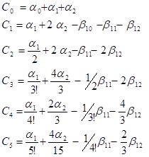 (5)
(5)
imposing accuracy of order 4 on Tn+2 to have
C0 = C1 = C2 = C3 = C4=0 and Tn+2 = 0(h5),
that is;
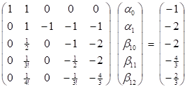
solving gives;
α0 = -1, α1= 0, b10 = 0.3333, b11 =1.3333 and b12 =0.333
putting these values into equation (2) gives two – step, first derivative method of equation of the form:
![]()
which coincides with Simpson’s rule (Lambert,1973).
Following the same pattern of derivation, the following variants of the two step multiderivative methods were derived:
Two – step second derivative method of the form:
![]()
Two – step third derivative method of the form:
![]()
Two – step fourth derivative method of the form:
![]()
Two – step fifth derivative method of the form:
![]()
Two – step sixth derivative method of the form:

Analysis of Absolute Stability and its Region
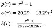
Letting the first and second characteristic polynomials of the resulting equations be ρ(r) and σ(r) respectively with h(r)=ρ(r)/σ(r), the RAS of each method was determined:
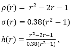
Two – step first derivative method of the form:
![]() ………………………… …………….. ……………………….. (2)
………………………… …………….. ……………………….. (2)
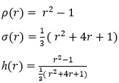
substituting r=eiϑ=cos ϑ+isin ϑ into h(r) gives
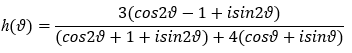
writing h(ϑ) in the form: x(ϑ)+iy(ϑ)
simplifying and setting the imaginary part to zero gives
![]()
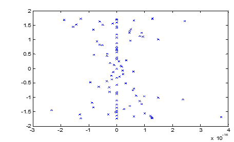
evaluating θ at an interval of 300 between 00 ≤ ϑ ≤ 1800, the interval of absolute stability is as given in the table
| ϑ | 00 | 300 | 600 | 900 | 1200 | 1500 | 1800 |
| x(ϑ) | 0.333 | 0.283 | 0.2 | -0.147 | -0.333 | -0.671 | -1 |
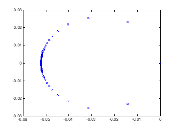
Figure 1: Region of A – stability for two- step first derivative method.
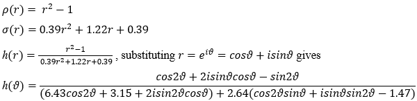
Two – step second derivative method of the form:
![]() …………………………. (3)
…………………………. (3)
substituting r = eiϑ= cos ϑ + isin ϑ gives
![]()
writing h(ϑ) jn the form: x(ϑ)+iy(ϑ)
simplifying and setting the imaginary part to zero gives
![]()
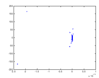
evaluating θ at an interval of 300 between 00 ≤ϑ ≤ 1800, the interval of absolute stability is as given in the table
| ϑ | 00 | 300 | 600 | 900 | 1200 | 1500 | 1800 |
| x(ϑ) | 0. | -0.507 | -1.341 | -1. 481 | -1.537 | -2.214 | -2.436 |
Figure 2: Region of A – stability for two- step second derivative method.
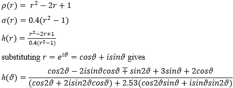
Two – step third derivative method of the form:
![]() …………………………………………….. (4)
…………………………………………….. (4)
writing h(ϑ) jn the form: x(ϑ)+iy(ϑ)
simplifying and setting the imaginary part to zero gives
![]()
evaluating θ at an interval of 300 between 00 ≤ϑ ≤ 1800, the interval of absolute stability is
as given in the table
| ϑ | 00 | 300 | 600 | 900 | 1200 | 1500 | 1800 |
| x(ϑ) | -2.742 | -2.061 | -1.335 | -1. 481 | 2.539 | 3.538 | 4 .632 |
Figure 3: Region of A – stability for two- step third derivative method.
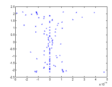
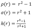
Two – step fourth derivative method of the form:
 ……………………………….. (5)
writing h(ϑ) jn the form: x(ϑ)+iy(ϑ)
simplifying and setting the imaginary part to zero gives
![]()
evaluating θ at an interval of 300 between 00≤ϑ≤1800, the interval of absolute stability is as given in the table
| ϑ | 00 | 300 | 600 | 900 | 1200 | 1500 | 1800 |
| x(ϑ) | -4.752 | -3.879 | -2.992 | -1. 769 | -1.209 | 0.822 | 0.457 |
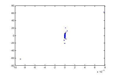
Figure 4: Region of A – stability for two- step fourth derivative method.
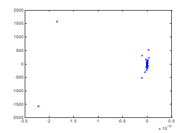
Two – step fifth derivative method of the form:
![]() …………………………………………. (6)
…………………………………………. (6)
substituting r=eiϑ=cosϑ+isinϑ gives
![]()
writing h(ϑ) jn the form: x(ϑ)+iy(ϑ)
simplifying and setting the imaginary part to zero gives
![]()
evaluating θ at an interval of 300 between 00≤ϑ≤1800, the interval of absolute stability is as given in the table
| ϑ | 00 | 300 | 600 | 900 | 1200 | 1500 | 1800 |
| x(ϑ) | -2.001 | -1.561 | -1.329 | 0. 458 | 0.853 | 1.352 | 1.963 |
Figure 5: Region of A – stability for two- step fifth derivative method.
Two – step sixth derivative method of the form:
 …………………… (7)
substituting r=eiϑ=cosϑ+isinϑ gives
writing h(ϑ) jn the form: x(ϑ)+iy(ϑ)
simplifying and setting the imaginary part to zero gives
![]()
evaluating θ at an interval of 300 between 00≤ϑ≤1800, the interval of absolute stability is as given in the table
| ϑ | 00 | 300 | 600 | 900 | 1200 | 1500 | 1800 |
| x(ϑ) | -0.048 | -0.041 | -0.039 | -0.034 | -0.029 | -0.024 | -0.019 |
Figure 6: Region of A – stability for two- step sixth derivative method.
IMPLEMENTATION
To access the convergence of the methods, the methods were used to solve sampled stiff initial value problem of first order ordinary differential equation:
![]()
Exact solution: y(x)=x3+e-10x the results are as shown in tables 1 and 2.
Table 1: Table of results showing Exact solution and all the Two – step Multiderivative Methods
| X | Exact Solution | K=2, L=1 | K=2, L=2 | K=2, L=3 | K=2, L=4 | K=2, L=5 | K=2, L=6 |
| 0.2 | 0.14333528323661271 | 0.34133333333333316 | 0.14029611111111112 | 0.14048944444444411 | 1.12799074074074100 | 0.14252412698412678 | 0.14245895214547660 |
| 0.4 | 0.08231563888873419 | 0.17511111111111102 | 0.08167432324845677 | 0.08148405204475303 | 1.31897920378943790 | 0.08213135977576212 | 0.08188996652823037 |
| 0.6 | 0.21847875217666643 | 0.25303703703703700 | 0.21863718377289668 | 0.21823785106621063 | 1.62285496328909470 | 0.21847838009047860 | 0.21808689735062664 |
| 0,8 | 0.51233546262790264 | 0.52434567901234574 | 0.51276873092641329 | 0.51221667067259680 | 2.08974566222867610 | 0.51237330278280269 | 0.51184076898280306 |
| 1.0 | 1.00004539992976250 | 1.00411522633744840 | 1.00064165398820020 | 0.99994872391069356 | 2.77004700691335780 | 1.00009020329884550 | 0.99941857722581540 |
| 1.2 | 1.72800614421235310 | 1.72937174211248300 | 1.72874484982807750 | 1.72791320235732800 | 3.71445654046030250 | 1.72805213091189590 | 1.72724177598923330 |
| 1.4 | 2.74400083152871850 | 2.74445724737082840 | 2.74487849604462620 | 2.74390849328473200 | 4.97401167144218630 | 2.74404701078017380 | 2.74309798933616330 |
| 1.6 | 4.09600011253517420 | 4.09615241579027600 | 4.09701616890056640 | 4.09590786900559410 | 6.60013249378768310 | 4.09604632220373070 | 4.09495864443054720 |
| 1.8 | 5.83200001522997800 | 5.83205080526342370 | 5.83315437422364090 | 5.83190778624525660 | 8.64467000159295120 | 5.83204622960112750 | 5.83081989711284530 |
| 2.0 | 8.00000000206115120 | 8.00001693508780680 | 8.00129264995810100 | 7.99990777527376280 | 11.1599603785529060 | 8.00004621714754550 | 7.99868123019424450 |
| 2.2 | 10.6480000002789430 | 10.6480056450292650 | 10.6494309350034850 | 10.6479077738192750 | 14.1988861273581720 | 10.6480462154727360 | 10.646542574092095 |
Table 2: Table of Errors of all the Multiderivative Methods when compared with the Exact solution
| X | K=2, L=1 | K=2, L=2 | K=2, L=3 | K=2, L=4 | K=2, L=5 | K=2, L=6 |
| 0.2 | 1.979981e-01 | 3.039172e-03 | 2.845839e-03 | 9.846555e-01 | 8.111563e-04 | 8.763311e-04 |
| 0.4 | 9.279547e-02 | 6.413156e-04 | 8.315868e-04 | 1.236664e+00 | 1.842791e-04 | 4.256724e-04 |
| 0.6 | 3.455828e-02 | 1.584316e-04 | 2.409011e-04 | 1.404376e+00 | 3.720862e-04 | 3.918548e-04 |
| 0,8 | 1.201022e-02 | 4.332683e-04 | 1.187920e-04 | 1.577410e+00 | 3.784015e-05 | 4.946936e-04 |
| 1.0 | 4.069826e-03 | 5.962541e-04 | 9.667602e-05 | 1.770002e+00 | 4.480337e-05 | 6.268227e-04 |
| 1.2 | 1.365598e-03 | 7.387056e-04 | 9.294186e-05 | 1.986450e+00 | 4.598670e-05 | 7.643682e-04 |
| 1.4 | 4.564158e-04 | 8.776645e-04 | 9.233824e-05 | 2.230011e+00 | 4.617925e-05 | 9.028422e-04 |
| 1.6 | 1.523033e-04 | 1.016056e-03 | 9.224353e-05 | 2.504132e+00 | 4.620967e-05 | 1.041468e-03 |
| 1.8 | 5.079003e-05 | 1.154359e-03 | 9.222898e-05 | 2.812670e+00 | 4.621437e-05 | 1.180118e-03 |
| 2.0 | 1.693303e-05 | 1.292648e-03 | 9.222679e-05 | 3.159960e+00 | 4.621509e-05 | 1.318772e-03 |
| 2.2 | 5.644750e-06 | 1.430935e-03 | 9.222646e-05 | 3.550886e+00 | 4.621519e-05 | 1.457426e-03 |
Figure 7: Graphical representation of Exact solution and Two – step first derivative method
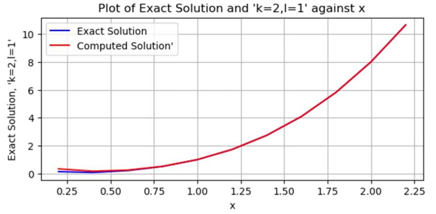
Figure 8: Graphical representation of Exact solution and Two – step second derivative method
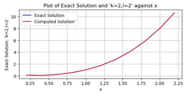
Figure 9: Graphical representation of Exact solution and Two – step third derivative method
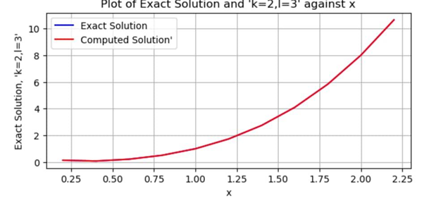
Figure 10: Graphical representation of Exact solution and Two – step fourth derivative method
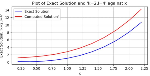
Figure 11: Graphical representation of Exact solution and Two – step fifth derivative method
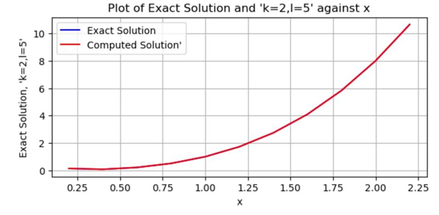
Figure 12: Graphical representation of Exact solution and Two – step sixth derivative method
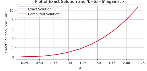
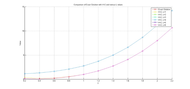
Figure 13: Graphical representation of Exact solution with all the methods .
DISCUSSION OF RESULTS AND CONCLUSION
Figures 1 – 6 showed that all the methods have reasonably wide region of A – stability except the two – step fourth derivative method (k=2, l=4) whose region did not extend to the left half of the complex plain. Since numerical methods that will solve stiff problems must be A – stable and possess wide region of A – stability, it is evident from Tables 1 and 2 why all the methods are accurate and convergent except the two – step fourth derivative method.
The graphical representation of the comparative analysis of the numerical results with the exact solution in Figures 7 – 12 also confirmed that a numerical method with poor region of absolute stability will not yield an accurate result and the result will not converge to the exact solution while on the other hand, a numerical method with reasonably wide region of absolute stability will yield a more accurate and convergent result when used to solve stiff initial value problems of ordinary differential equations.
REFERENCES
- Butcher, J. (2008). Numerical Methods for Ordinary Differential Equations (2nd ed.). John Wiley and Sons Ltd, West Sussex
- Famurewa O. K., Ogunrinde R.B. and Dare J.R. (2019). Variation of Step – size and the Effect on the Accuracy of an Implicit One – step Multiderivative method for Solving Non – Stiff and Stiff O.D.Es. International Journal of latest Technology in Engineering, Management & Applied Science (IJLTEMAS) 8(11) (2019) 24 – 28 \1SSN 2278 – 2540.
- Hairer, E., Norset, S. & Wanner, G. (2008). Solving Ordinary Differential Equations I: Nonstiff Problems. BIT, 18: 475-489.
- Ibijola E.A and Ogunrinde R.B. (2010). On a New Numerical Scheme for the Solution of Initial Value Problems (Ivps) In Ordinary Differential Equation. Aust. J. Basic & Appl. Sci., 4(10): 5277-5282.
- Ogunrinde R.B. and Fadugba (2012). Development of a New Scheme for the Solution of Initial Value Problems in Ordinary Differential Equations. Journal of Mathematics 2(2): 24 – 29.
- Olumurewa O. K. (2020). Investigating Absolute Stability and its Region of an Implicit Linear Multiderivative Scheme for Solving Stiff Ordinary Differential Equations. International Journal of Applied Science and Mathematical Theory (IJASMT) Vol. 6 No 3 (2020) 1 – 7 E -ISSN 2489 – 009X P – ISSN 2695 – 1908
- Süli, Endre and Mayers, David (2003), An Introduction to Numerical Analysis, Cambrige University Press, ISBN 0-521 -00794-1.