Algebraic solution of the Quantum Harmonic Oscillator
- Joseph Hlongwane
- 62-75
- Apr 29, 2024
- Mathematics
Algebraic Solution of the Quantum Harmonic Oscillator
Joseph Hlongwane
Faculty of Science and Technology Education, National University of Science and Technology, Zimbabwe
DOI: https://doi.org/10.51584/IJRIAS.2024.90405
Received: 09 March 2024; Accepted: 28 March 2024; Published: 29 April 2024
ABSTRACT
The Wave-particle duality and the Schrodinger cat paradox pose important notions on quantum mechanical systems, in which a quantum system can exist in two physically opposite or distinct states. This motivates scientists from the days of Louis de Broglie to confidently look at matter as having a dual nature, which is a physical particle that can also be visualized as a wave entity. This paper seeks to provide an elegant method of solving the time-independent Schrodinger Equation (TISE) for a quantum simple harmonic oscillator (QSHO). A fully algebraic method is presented, the paper explains in detail how simple algebra, coupled with basic quantum mechanical operator commutation algebra can be employed to solve the TISE without resorting to complicated mathematical methods of solving second-order differential equations. The construction of the Hamiltonian is explained and an analogy between the classical simple harmonic oscillator (CSHO) and the QSHO is drawn to develop the solution method. The action of creation and annihilation operators on wave functions is exploited to generate states with higher and lower energies respectively and to generate a Hamiltonian that can act on a system and generate required quantum states. The aim is to generate the ground state of the QSHO and its associated energy value. From this state, other higher energy states can be generated by the action of the creation operator. The use of algebraic methods has been seen to be versatile as it does not explicitly rely on any particular basis or coordinate system. The method allows operators to be manipulated in different bases for example the momentum operator can be given as P ̂ x=-iℏ (∂/∂x) in a spatial coordinate basis or as a pure number p ̂ =p in the momentum basis.
Keywords: quantum harmonic oscillator, quantum operators, commutator, normalization, Schrödinger equation, algebraic solution
INTRODUCTION
This paper serves to present a simple method of solving the TISE for the QSHO. The QSHO draws its analogy to the classical simple harmonic oscillator (CSHO). Common examples of CSHOs are the simple pendulum and the mass-spring system. The potential energy expression of the mass-spring system is employed in the quantum model outlined in this paper. Complicated mathematical manipulations have been avoided in preference to simpler algebraic mathematical methods to assist all students with different mathematical backgrounds to be able to follow and understand the solution. The constructivist learning theory is employed throughout the discussion, that is we start from the known and build up knowledge towards what we want to know which is at present unknown (Schunk, 2012). Effort shave been made to bring out the ideas of quantum mechanics without clouding the student or reader with too much mathematics. This paper also seeks to bring out the unity and relationship between several topics in Physics so that it is clear that Physics as a discipline is one unified body of knowledge and not a collection of independent scientific ideas.
It would be misleading to claim that mathematical methods can be used to accurately describe a physical system. To construct a mathematical model of a physical system, several assumptions and conditions are made to make the system mathematically solvable. These assumptions may not make sense or may not be applicable physically. On this note, this paper does not claim to provide a 100% accurate solution. Mathematical models presented are tools that help to explain the solution of the TISE for the QSHO by drawing an analogy with a physical CSHO (Slavnov, 2006).
The paper has been broken down into several sub-topics that build up to the ultimate goal of solving the TISE. The Hamiltonian operator and the ladder operators are introduced and later the Hamiltonian is expressed in terms of the ladder operators and applied to a normalised wave function to obtain the ground state, excited states and their associated energies.
THE HAMILTONIAN
The Hamiltonian is a quantum mechanical operator representing a system’s total energy (E). It is the summation of the kinetic and potential energies of the individual particles in any given system. Microscopic particles like electrons, protons, photons, neutrons, and several fundamental particles in nature and atoms can be modelled as waves according to the wave-particle duality coined by Louis de Broglie (Zeilinger, 1999).
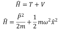
We begin by introducing the Hamiltonian, adopted by Wheeler (2012):
H ̂=T+V (1)
But the potential energy(pe) or V is that of a classical simple harmonic oscillator (mass-spring system). The QHSO can be modelled as a classical oscillator comprising a mass attached to a spring. This system has a potential given by the expression:
V(x)= 1/2(kx2) (2)
It is widely believed that classical physics is merely a restricted instance of quantum physics, implying that several classical phenomena possess quantum physics analogues. As a result, this encourages the analogous approach of treating quantum and classical systems alike. Hence, this paper is confident in applying the classical potential energy equation to the QSHO. (Slavnov, 2005).
If we substitute k=mω2 from a classical mass-spring system SHO. Equation (2) becomes:
V(x)=1/2 (mω2 x ̂2) (3)
where m is the mass of the oscillator, x is its displacement from the equilibrium position and omega (ω) is the angular velocity or angular frequency.
The general formula for kinetic energy (T) is:
ke=1/2 (mv2) (4)
But the momentum of a particle p=mv where v is the velocity of the particle. Now from p=mv it follows that p2=m2v2 therefore mv2=p2/m
Therefore it follows that kinetic energy can be expressed in terms of momentum. Note that in quantum mechanics the momentum and displacement operators play pivotal roles in quantum systems.
ke=1/2 (p2/m) (5)
In quantum mechanics, the momentum operator is given as:
P ̂=-iℏ ∂/∂x (6)
Where ℏ is the reduced Planck constant and ∂/∂x is the partial derivative with respect to displacement along the x coordinate.
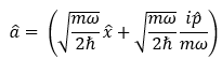
Putting everything together, the Hamiltonian of the QSHO can be expressed as:
 (6a)
(6a)
Substituting equation (6) for P ̂ in equation (6a) we obtain the Hamiltonian in its differential form:
![]() (7)
(7)
Equation (7) can be alternatively presented as:
![]() (8)
(8)
Where V(x) represents an arbitrary potential for example a magnetic, electrical or mechanical potential.
According to the wave-particle duality, particles exhibit wave-like behaviour which is more prevalent at microscopic or nanoscopic levels. Quantum particles are thus modelled as waves and represented by the Schrodinger wave equation. The particles are examples of quantum states denoted by the wave function ψ(x), psi as a function of an arbitrary coordinate, say x (Schleich, 2016).
THE TIME-INDEPENDENT SCHRODINGER EQUATION
The ground and excited wave states of the QSHO and their corresponding energies can be determined by solving the time-independent Schrödinger equation:
![]() (9)
(9)
The Schrödinger equation is an eigenvalue equation. If the Hamiltonian operates on a state psi it generates a state with higher energy, the same state multiplied by eigenvalue E, a real number corresponding to the total energy of the system.
Substituting (8) into (9) we obtain:
![]() (10)
(10)
The major aim of this paper is to solve the Schrodinger equation (10) without going through the rig our of solving the second-order differential equation and obtain the possible quantum states ψ(x) of the QSHO and associated energy values.
According to the Schrödinger Cat paradox, a quantum system can exist in more than one state at any given time, this is motivated by Erwin Schrödinger when he asserted that a cat can be both alive and dead inside a box with a radioactive substance. The researcher uses this paradox to suggest that our state ψ(x) can exist in several physical and different states or conditions at any given time. Given that these states are waves one is driven to believe that these states could be superposed on each other. (Schrodinger, 1935).
LADDER OPERATORS
Ladder operators are so-called because they either raise or lower the energy state of a quantum system just like what a physical ladder does in assisting to hoist or lower a physical body. The raising operator (a ̂†) acts on a quantum state and generates a new state of higher energy by a factor of whilst thelowering operator (a ̂) can generate lower energy states by the same factor. These operators are also called annihilation and creation operators because they can destroy or create a quantum of energy respectively.
The combination of these operators provides an eloquent method for solving the harmonic oscillator problem and several other classical and quantum systems (Kelley and Leventhal, 2017).
The mathematical manipulations for the creation and annihilation operators for particles with integral spins (bosons)for example gluons, photons, gravitons and Higgs bosons and that for particles with half-integer spins (fermions) for example neutrons, electrons and protons and protons are different. For example, the commutation relation for the creation and annihilation operators for similar bosonic systems is equal to one, while all other commutators are zero. However, for fermions the mathematics is similar to that for the QSHO and it involves anti-commutators instead of commutators in the case of bosons (Feynman, 1998).
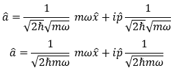
The Lowering (Annihilation) Operator
![]() (11)
(11)
We want the lowering operator to act on a function, but it is very difficult and complicated to use it in the form of equation (11), we therefore transform it into a more user-friendly form. We begin by opening the bracket.
The square root signs affect both numerators and denominators therefore we can root the numerators and denominators separately for simpler calculations:
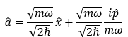
To simplify the expression we play a mathematical trick, multiplying the numerators and denominators of both fractions by the same constant (mω in this case) does not change anything mathematically but will help us simplify our expression.
In mathematics ![]() therefore:
therefore:
Factoring out common terms and re-arranging for convenience results in:
![]() (12)
(12)
The Raising (Creation) Operator
![]() (13)
(13)
Again, if we open the brackets and follow the above steps on dealing with the lowering operator and also multiply the numerators and denominators on the right-hand side by and simplify, we get an alternative expression for the creation operator:
![]() (14)
(14)
The Quantum Energy Term
It should be noted that ℏω is an energy term. It was argued earlier that the ladder operators either create or annihilate new states with energy values differing by a constant factor of ℏω . This sub-section tends to prove that ℏω is indeed an energy term.
The energy of a quantum particle is generally given by the equation (15) where all terms have their usual meanings in Physics:
E=hf (15)
The angular frequency of an oscillating particleis ω=2πf, therefore:
f=ω/2π (16)
Substituting (16) into (15) we get:
E=hω/2π (17)
Where ℏ is the reduced Planck’s constant:
h/2π=ℏ (18)
Therefore by substituting (18) into (17), we obtain an alternative energy term which can be expressed as:
E=hω/2π=ℏω (19)s
Generating a New Hamiltonian from Ladder Operators
To solve equation (10) we first multiply both ladder operators to obtain their product. This will lead us to the generation of a new Hamiltonian which will take care of all possible quantum states that can exist simultaneously as espoused by the Schrodinger Cat paradox.
Now:
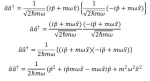
Rearranging the terms enclosed in the bracket,
![]() (20)
(20)
It is very important to note that p ̂ and x ̂ are not constants but are operators. We therefore treat them according to operator commutation rules. Their commutation relation is given by the expression [x ̂, p ̂] which is expanded as: =![]() (20a)
(20a)
If the order of these commutators is reversed, then ![]() (21)
(21)
Substituting equation (21) into (20) we get:
![]()
But from (21) [p ̂, x ̂] =-iℏ therefore
![]() (22)
(22)
Dividing each term in braces by 2ℏmω or multiplying every term by 1/2ℏmω
![]()
Factoring out 1/ℏω and noting that i2=-1 gives:
![]() (23)
(23)
Comparison of (23) with (6a) ![]() shows that the first two terms inside the brackets give the Hamiltonian of the system therefore (23) can be re-written as:
shows that the first two terms inside the brackets give the Hamiltonian of the system therefore (23) can be re-written as:
![]() (24)
(24)
Simplification of (24) results in:
![]() (25)
(25)
We rearrange this equation to get a new expression for the Hamiltonian:
![]() (26)
(26)
But from (9) we stated that H ̂ψ(x)=Eψ(x). This means that when the Hamiltonian acts on a quantum state it yields a new state with an energy value of E. Now if this Hamiltonian acts on a state already acted upon by a raising or lowering operator it will yield a state with a higher or lower energy than the original state respectively.
Energy Levels for a Harmonic Oscillator
The potential well of a Harmonic Oscillator is parabolic and thus maximum possible energy is infinite (increases unbounded up the vertical axes). Still, there must be the lowest possible energy value (the zero point energy in Fig.1.) which corresponds to the lowest energy state which is called the ground state (ψ0). See Fig.1 for the diagram of the potential well.
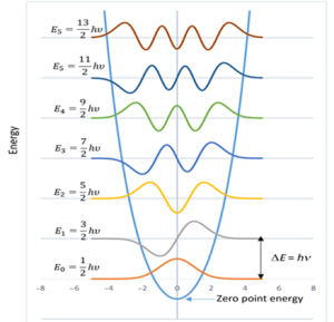
Fig .1. Potential well for a classical Harmonic Oscillator (Browne, 2020)
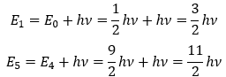
Energy is a quantized phenomenon, meaning that it exists in discrete packages known as quanta. These quanta have a specific value that can be determined by the equation E=hf, where E represents energy, h is Planck’s constant, and f represents frequency. In Fig.1, the frequency symbol “f” is replaced with the Greek letter “ν” (nu) while the physics and mathematics remain the same. As you move up the energy levels (E0, E1, E2…and beyond.), there is an increase in the steps of hv. This quantization phenomenon is a fundamental aspect of quantum mechanics, which is essential in understanding the behaviour of particles at the atomic and subatomic levels.
The general equation for the energy of a QHO is given by (39) as
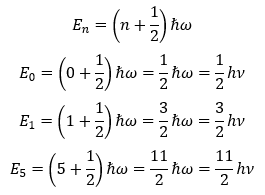
Note that from (15) and (19) E=hf=ℏω=hν therefore the energy values are seen to be increasing by this constant value.
As an example: E0=1/2 hν
In the realm of quantum mechanics (QM), the precise position and momentum of a quantum particle cannot be determined with certainty due to the probabilistic nature of QM. However, their mean or expected values can be calculated. Fig.1. illustrates a symmetric potential well around x=0, implying that the probability of finding the particle at a point where x>0 is equivalent to that where x<0. As a result, the mean values of displacement and momentum are both zero.
In classical physics, momentum (P) can be computed as P=mv, where m represents the mass of the particle and v reflects its velocity. If the momentum is zero, the classical particle is at rest with v=0, as the mass of an existing classical particle cannot be zero. In contrast, zero momentum for a quantum particle denotes an average value of all momenta in the positive and negative x directions. An oscillating quantum particle moves back and forth through the equilibrium position, without necessarily being at rest. If the particle is not at rest, then it must possess some energy. If it is not being translated to other points, it should be vibrating around x=0, thereby having vibrational energy at this point.
The lowest energy a quantum particle can possess is referred to as the zero point energy or ground state energy, which is expressed in equation (36). This differs from the case of a classical particle, where the minimum energy can be zero for a stationary particle.
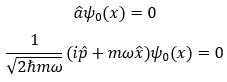
It then follows that if the lowering operator acts on the ground state it will produce a state with zero energy, this is the lowest possible observable energy value because we cannot observe negative energy values. Therefore no state can physically exist with negative energy (note that mathematically this is possible). The ground state is the lowest energy state that can exist.
Consider the following eigenvalue equation:
a ̂ψ0 (x)=0 (27)
SOLUTION OF THE SCHRÖDINGER EQUATION
In quantum mechanics, Schrödinger’s cat paradox is a quantum phenomenon analogous to wave-particle superposition. However, when an observation is made or measurement is taken on this system, the wave function collapses or is reduced to only one of the possible states, the particular observation. This suggests that when an observation is made by whatever instrument is used, the superposition of states disappears, and the system is seen in only one of its several possible states. in other words, the actual act of measuring or observing a quantum system disturbs its actual reality and gives the observer the impression of a single state function corresponding to what is under investigation (Schlosshauer and Maximilian, 2005; Giacosa, 2014).
A hypothetical cat may be considered to be simultaneously both alive and dead while it is unobserved in a closed box with a substance likely able to kill it. Once the box is opened and the cat is observed, there’s a 50% chance of it being alive or dead. This summarises the phenomenon of wave-function collapse, a wave-function can be observed in one of its possible states at a time, either the ground state or one of the excited states (Peres, 1993).
Our task in this section is to solve the Schrödinger equation and find an explicit expression for the ground state. The action of the creation operator on the ground state can yield higher energy excited states.
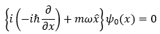
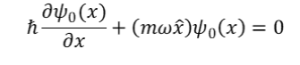
We start from (27) and substitute for from equation (12)
Multiplying both sides by √2ℏmω gives us:
![]() (28)
(28)
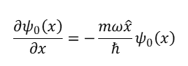
But from (6) P ̂=-iℏ ∂/∂x
Thus substituting (6) into (28) we obtain:
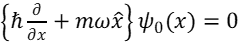
If we multiply the contents of the bracket by i we obtain the expression:
![]() (28a)
(28a)
Note that =√(-1), then i2=-1and (-1)2=1, therefore simplifying (28a) gives:
 (28b)
(28b)
Simplifying the left-hand side of the equation (28b) by opening the braces we get:
 (28c)
(28c)
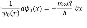
Dividing every term on both sides of equation (28c) by ℏ and re-arranging the equation gives:
Collecting like terms and grouping them on one side results in the equation:
 (28d)
(28d)
Integrating both sides of the equation (28d) gives:
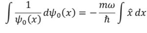 (29)
(29)
Two of the fundamental rules for integration in mathematics state that ∫1/x dx=lnx+c and ∫xn dx= (xn+1/(n+1))+c where c is an arbitrary constant of integration. There fore the result of integrating equation (29) is:
 (29a)
(29a)
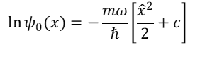
The application of mathematical rules for natural logarithms on both sides of the equation (raising every term to base e) gives us:
 (29b)
(29b)
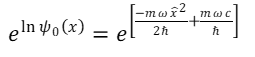
Taking anti-logarithms on both sidesof equation (29b) results in:
 (29c)
(29c)
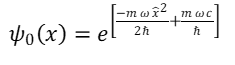
But generally a(x+b)=ax ab , therefore equation (29c) becomes:
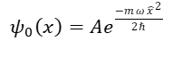

Since c, m, and ℏ are all constants, it follows that emωc/ℏ is a constant, let us call it A.
Therefore equation (29c) can be re-written as:
 (30)
(30)
‘A’ is the scalar multiple required to make the given wave function adhere to the normalization condition explained in sub-section 8.1 below.
Normalisation
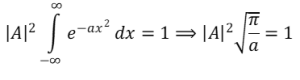
We now use the standard normalisation expression (31) to normalise (30) so that we can solve it easily. The normalization condition states that the integral of the square of the wave function in all space must be equal to one. This means that the particle represented by the wave function must be present at some position in space along a particular axis, in this case, the x-axis (Swenson and Hermanson, 1972).
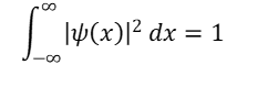 (31)
(31)
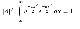
Substituting for the wave function (30) in the equation (31) we obtain:
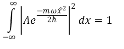 (32)
(32)
Equation (32) Can be simplified by taking out the constant A to give:
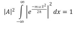 (32a)
(32a)
This equation can be rewritten to match the standard integrals in QM whose general solutions are known. Note that m, w, and ℏ are constants. They can be grouped and represented by an arbitrary constant a, where
thus equation (32a) becomes:
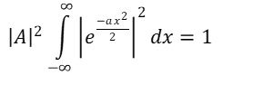 (32b)
(32b)
We can expand the term inside the modulus brackets
 (32c)
(32c)
This equation can be simplified by the application of the law for indices, e is raised to a power equal to the sum of the individual powers:
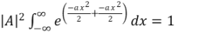 (32d)
(32d)
We clear the brackets to obtain the final expression:
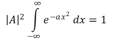 (33)
(33)
But from given standard integral equations, the general solution of such equations as (33) is of the form:
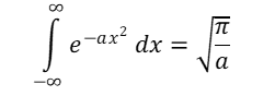 (34)
(34)
Comparing the equation we generated (33) to the standard equation (34) shows that:
 (35)
(35)
But our =mω/ℏ. Substituting for ‘a’ in equation (35) results in:
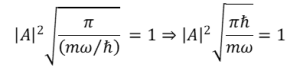 (35a)
(35a)
We clear the square root sign by squaring every term in (35a) to get:
(A4 πℏ)/mω=1 (35b)
To calculate the normalization constant A, we make it the subject of the formula in (35b): (A4 πℏ)/mω=1⇒A4=mω/πℏ, taking the fourth root on both sides of this equation gives us:
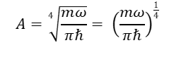 (36)
(36)
If we substitute this expression for A into equation (30) we obtain the required expression for the ground state. This wave function contains all the information required to fully understand the behaviour and characteristics of the quantum particle represented by the wave function. (Dekker, 1981).It is worth noting that the wave function can collapse into any state corresponding to any particular observable (Giacosa, 2014).
The general expression of the ground state of the QSHO along coordinate x is therefore:
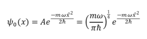
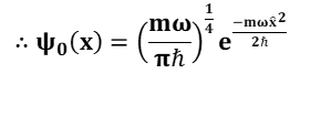 (37)
(37)
ENERGY VALUES ASSOCIATED WITH THE GROUND STATE
If the raising operator acts on the ground state, excited states of higher energy will be obtained.
The action of the Hamiltonian on a quantum state produces a different energy state and if it acts on the ground state it would yield a state of lowest observable energy(E0), let us calculate this energy by applying equation (9) to the ground state. The solution of the Schrodinger equation shows that energy levels of a harmonic oscillator are quantized, they are not arbitrarily continuous and can only have particular discrete values. (Triana and Fajardo, 2011).
H ̂ ψ0 (x)=E0 ψ0 (x)
The Hamiltonian can be re-stated according to equation (26) in terms of the ladder operators and plugged into Schrödinger’s equation:
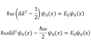
Take note of the order in which the operators appear. If the raising operator first acts on the ground state it will generate a higher energy state say ψ1 (x) When the lowering operator next acts on the new state ψ1 (x) it will lower it back to the initial ground state.
(a) ̂ † ψ0 (x) = ψ1 (x); a ̂ ψ1 (x)= ψ0 (x),
Hence:
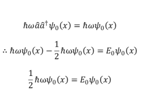
Taking out ψ0 (x) on both sides we obtain an expression for the ground state energy level:
E0=1/2 ℏω (38)
If the raising operator acts on a quantum state with this amount of energy, the energy will be raised to a higher level generally expressed as:
En=(n+1/2)ℏω (39)
It is of note that applying the Hamiltonian repeatedly on a ̂ † ψ0 (x) will give states of higher energy than the ground state.
CONCLUSION
The present paper introduces an elegant and straightforward algebraic approach to solving the time-independent Schrodinger Equation for a quantum simple harmonic oscillator. The paper aims to generate the ground state and its associated energy value by exploiting basic quantum mechanical operator commutation algebra and the action of creation and annihilation operators on wave functions. The Hamiltonian operator and the ladder operators are introduced, and the Hamiltonian is expressed in terms of the ladder operators and applied to a normalized wave function to obtain the ground state, excited states, and their corresponding energies. The algebraic method provides a versatile and reliable solution, as it does not require any particular basis or coordinate system. Furthermore, the paper highlights the unity and interconnectedness of several topics in Physics, emphasizing that Physics is a unified discipline rather than a collection of disparate scientific ideas. This paper is a valuable resource for students and researchers seeking to comprehend quantum mechanics without resorting to complex mathematical methods. The approach presented in this paper is both accessible and comprehensive, making it an excellent tool for those interested in furthering their knowledge in this field.
This paper presents a method for solving the time-independent Schrodinger Equation for a quantum simple harmonic oscillator. The approach is based on using basic quantum mechanics operator commutation algebra and the Hamiltonian, creation and annihilation operators on wave functions. By applying these operators, the method generates the ground state and its associated energy value, and further action of these operators generates excited quantum states. Notably, this method does not rely on any particular basis or coordinate system, making it a versatile approach.
The paper emphasizes the unification of various topics in Physics, highlighting that Physics is a unified body of knowledge. The theories of wave-particle duality by de Broglie and the Schrodinger cat paradox are used to draw important analogies between classical and quantum mechanics, which are then applied to model a solution to the TISE.
This paper can serve as a useful tool for students and researchers interested in understanding quantum mechanics without the need for complex mathematical manipulations.
REFERENCES
- Browne, W. (2020). Molecular Inorganic Chemistry. Retrieved from Practical Approaches to Biological Inorganic Chemistry: https://doi.org/10.1016/B978-0-444-64225-7.00008-0
- Dekker, H. (1981). Classical and quantum mechanics of the damped harmonic oscillator. Physics Reports, 80(1), 1-110.
- Feynman, R. (1998). Statistical Mechanics: A Set of Lectures 2nd Ed. Reading, Massachusetts: Addison-Wesley.
- Giacosa, F. (2014). On unitary evolution and collapse in quantum mechanics. Quanta. 3(1), 156-170.
- Kelly, J., & Leventhal, J. (2017). Ladder Operators for the Harmonic Oscillator. Retrieved from Problems in Classical and Quantum Mechanics, Springer, Cham: https://doi.org/10.1007/978-3-319-4666-4 7
- Peres, A. (1993). Quantum Theory. Concepts and Methods. Kluwer, 373-374.
- Schleich, W. (2016). Wave-Particle Dualism in Action. Optics in Our Time.
- Schlosshauer, M. (2005). Decoherence, the measurement problem, and interpretations of quantum mechanics. Rev. Mod. Phys. 76(4), 1267-1305.
- Schrodinger, E. (1935). Die gegenwartige Situation in der Quantenmechanik(The present situation in quantum mechanics). Naturwissenschaften. 23(48), 807-812.
- Schrodinger, E. (1935). Die gegenwartige Situation in der Quantenmechanik(The present situation in quantum mechanics). Naturwissenschaften. 23(48), 807-812.
- Slavnov, D. (2005). Necessary and Sufficient Postulates of Quantum Mechanics. Theoretical and Mathematical Physics, 142(3), 431-446.
- Slavnov, D. (2006). The possibility of reconciling quantum mechanics with classical probability theory. Theoretical Mathematical Physics 149, 1690-1701.
- Swenson, R., & Hermanson, J. (1972). Energy quantization and the simple harmonic oscillator. American Journal of Physics, 40(9), 1258-1260.
- Swenson, R., & Hermanson, J. (1972). Energy quantization and the simple harmonic oscillator. American Journal of Physics, 40(9), 1258-1260.
- Triana, C., & Fajardo, F. (2011). The influence of spring length on the physical parameters of simple harmonic motion. European Journal of Physics, 33(i), 219.
- Wheeler, J., & Zurek, W. (1983). Quantum Theory and Measurement. Princeton, NJ: Princeton University Press.
- Zeilinger, A. (1999). Experiment and the Foundations of Quantum Physics. Reviews of Modern Physics, 71(2), S288-S297.