Maternal Health Risk Prediction Using Machine Learning Methods
- Ibewesi, MaryJane Chinyere
- Uzuke Chinwendu Alice
- 376-393
- May 21, 2024
- Health
Maternal Health Risk Prediction Using Machine Learning Methods
Ibewesi, MaryJane Chinyere and *Uzuke Chinwendu Alice
Department of Statistics
Nnamdi Azikiwe University, Awka Nigeria
*Corresponding Author
DOI: https://doi.org/10.51584/IJRIAS.2024.904027
Received: 03 April 2024; Accepted: 10 April 2024; Published: 21 May 2024
ABSTRACT
This work employed machine learning methods – decision tree algorithm, support vector machine (SVM) and logistic regression to predict health risk outcome of pregnant women based on their vital signs. The aim was to determine which of the model most suitable for the prediction of health risk for any pregnant woman. Evaluation of the methods were done using Accuracy, Precision, F1-Score and recall. The results revealed that the Decision tree model achieved the highest accuracy of 0.8669 (86.99%), that indicates correct prediction in 86.99% of the cases. Also, it achieved the highest precision for all the risk categories (high_risk, low_risk and mid_risk) with values (87%, 86% and 75% respectively) implying lower likelihood of false positive predictions for all risk categories. The Decision Tree model appears to be a promising approach for predicting the impact of vital signs on health risk of pregnant mothers. It exhibited high precision, high recall (sensitivity) and a balanced F1-score, suggesting accurate predictions with very low rate of false positives.
Keywords: machine learning, decision tree, support vector machine, accuracy, precision.
INTRODUCTION
Analysis of big data by machine learning offers considerable advantages for assimilation and evaluation of large amounts of complex health-care data. Ngiam and Khor (2019) observed that the advantages of using machine learning include flexibility and scalability when compared with the traditional biostatistics methods, and this makes it deployable for many tasks, such as risk stratification, diagnosis and classification, and survival predictions. They also observed that the machine learning algorithms has the ability to analyse diverse data types (eg, demographic data, laboratory findings, imaging data, and doctors’ free-text notes) and how to incorporate them into predictions for disease risk, diagnosis, prognosis, and appropriate treatments. Despite these advantages, the application of machine learning in health-care delivery also presents unique challenges that require data pre-processing and model training.
The use of Machine Learning in pregnancy diseases and complications is quite recent, and has increased over the last few years. The applications are varied and point not only to the diagnosis, but also to the management, treatment, and pathophysiological understanding of perinatal alterations. Facing the challenges that come with working with different types of data, the handling of increasingly large amounts of information, the development of emerging technologies, and the need of translational studies, it is expected that the use of ML continues growing in the field of obstetrics and gynaecology (Mennickent, 2023)
Analysis of big data by machine learning offers considerable advantages for assimilation and evaluation of large amounts of complex health-care data. Ngiam and Khor (2019) observed that the advantages of using machine learning include flexibility and scalability when compared with the traditional biostatistics methods, and this makes it deployable for many tasks, such as risk stratification, diagnosis and classification, and survival predictions. They also observed that the machine learning algorithms has the ability to analyse diverse data types (eg, demographic data, laboratory findings, imaging data, and doctors’ free-text notes) and how to incorporate them into predictions for disease risk, diagnosis, prognosis, and appropriate treatments. Despite these advantages, the application of machine learning in health-care delivery also presents unique challenges that require data pre-processing and model training (Mohd et al 2022).
A deep learning model can also be used by healthcare organizations and pharmaceutical companies to identify relevant information in data that could lead to drug discovery, the development of new drugs by pharmaceutical companies and new treatments for diseases and also to improve the efficiency of healthcare leading to cost savings by developing better algorithms for managing patient records or scheduling appointments. This type of machine learning could potentially help to reduce the amount of time and resources. (Seth, 2023, Macrohon et al 2022)
Vital signs are considered vital to the rapid assessment of the patient when it is necessary to determine major changes in the patient’s basic physiological functioning. The vital signs include the assessment of the pulse, body temperature, respirations, blood pressure and oxygen saturation, which is the newest of all the vital signs.
The most common causes of maternal mortality are haemorrhage, sepsis and hypertensive disorders. There are established, effective solutions to these complications, however challenges remain in identifying who is at greatest risk and ensuring that interventions are delivered early when they have the greatest potential to benefit. Vital signs measurement remains a vital first step in detecting pregnancy abnormalities in order to initiate timely treatments that can save lives. Measuring vital signs is the first step in identifying women at risk. Overstretched or poorly trained staff and inadequate access to accurate, reliable equipment to measure vital signs can potentially result in delayed treatment initiation (Matthew et al 2016). Early warning systems may help alert users to identify patients at risk, especially where novel technologies can improve usability by automating calculations and alerting users to abnormalities. This may be of greatest benefit in under-resourced settings where task-sharing is common and early identification of complications can allow for prioritisation of life-saving interventions (Marques et al 2021). They further highlighted the challenges of accurate vital sign measurement in pregnancy and identified innovations which may improve detection of pregnancy complications. Failure to recognize and act on deteriorating vital signs in a timely manner contributed to avoidable maternal deaths. Strategies to improve timely recognition of women who require intervention to treat life-threatening pregnancy complications may prevent morbidity and mortality (Rescinito et al 2023). This study investigates the how Vital Signs influence health risk among pregnant mothers by examining the relationships between vital signs and their health risk levels. This will help uncover insights that contribute to more informed risk assessment strategies and personalized health management. Especially in low-resource settings, where the burden of disease from preventable conditions is so great and accessing appropriate care is critical. Inadequate access to accurate, reliable equipment in combination with strain on trained health care providers can lead to delay in recognition of pregnancy complications (Vousden, 2018)
METHODOLOGY
Decision Trees
They are graphical models that split the input space into regions based on some features. Each node in the tree represents a test on a feature, and each branch represents an outcome of the test. The leaf nodes represent the class labels or probabilities. To build a decision tree, one needs to choose a splitting criterion (such as entropy or Gini index), a stopping criterion (such as maximum depth or minimum number of samples), and a pruning method (such as reduced error pruning or cost complexity pruning). The equation for entropy as stated in Tan et al (2014) is given by:
\( H(S) = -\sum_{i=1}^{c} p_i \log_2 p_i \) (1)
where \( S \) is a set of samples, \( c \) is the number of classes, and \( p_i \) is the proportion of samples belonging to class \( i \) in \( S \). The equation for the Gini index is given by:
\( G(S) = 1 – \sum_{i=1}^{c} p_i^2 \) (2)
where the symbols have the same meaning as above. A lower value of entropy or Gini index indicates a higher purity of the set. To split a node, one chooses the feature and the threshold that maximizes the information gain or minimizes the impurity decrease. The information gain is defined as:
\( IG(S, A) = H(S) – \sum_{\nu \in Values(A)} \frac{S_\nu}{S} H(S_\nu) \) (3)
where \( A \) is a feature, \( Values(A) \) is the set of possible values for \( A \), and \( S_\nu \) is the subset of samples where \( A = \nu \). The impurity decrease is defined as:
\( \Delta I(S, A) = G(S) – \sum_{\nu \in Values(A)} \frac{S_\nu}{S} G(S_\nu) \) (4)
The symbols in equation (4) have the same meaning as in (3). To stop growing the tree, one can use a predefined maximum depth, a minimum number of samples at each node, or a minimum information gain or impurity decrease threshold. To prune the tree, one can remove nodes that do not improve the accuracy or complexity of the tree on a validation set or based on a cost function (De Cock et al. 2019).
Support Vector Machines (SVM)
Support Vector Machines, according to Abe (2005), aim to find a hyperplane that best separates classes in a higher-dimensional space. The margin between the hyperplane and the support vectors is maximized. Support vector machines are models that find a hyperplane that separates the data into two classes with maximum margin. The hyperplane is defined by a weight vector \( w \) and a bias term \( b \) such that:
\( w^T x + b = 0 \) (5)
where \( x \) is an input vector. The margin is defined by two parallel hyperplanes that pass through the closest points to the separating hyperplane such that:
\( w^T x + b = 1 \) (6)
and
\( w^T x + b = -1 \) (7)
The distance between these two hyperplanes is \( \frac{2}{||w||} \), so maximizing the margin is equivalent to minimizing \( ||w|| \). The closest points to the separating hyperplane are called support vectors and they satisfy:
\( y_i (w^T x_i + b) = 1 \) (8)
where \( y_i \) is the class label of \( x_i \), either +1 or -1. To find the optimal \( w \) and \( b \), one needs to solve the following optimization problem:
\( \min_{w, b} \frac{1}{2} ||w||^2 \) (9)
subject to:
\( y_i (w^T x_i + b) \geq 1, \, i = 1, \ldots, n \) (10)
where \( n \) is the number of samples. This is a convex quadratic programming problem that can be solved using Lagrange multipliers and Karush-Kuhn-Tucker conditions. The solution can be expressed in terms of the support vectors and their corresponding Lagrange multipliers \( \alpha_i \) such that:
\( w = \sum_{i=1}^{n} \alpha_i y_i x_i \) (11)
and
\( b = y_j – w^T x_j \) (12)
where \( j \) is any index of a support vector. The class prediction for a new input \( x \) is given by:
\( y = \text{sign}(w^T x + b) = \text{sign}\left( \sum_{i=1}^{n} \alpha_i y_i x_i^T x + b \right) \) (13)
Support vector machines can handle nonlinearly separable data by using a kernel function that maps the input to a higher-dimensional space where the data is linearly separable. A kernel function is a function that computes the inner product of two vectors in the feature space without explicitly mapping them such that:
\( \kappa(x_i, x_j) = \phi(x_i)^T \phi(x_j) \) (14)
where \( \phi \) is the mapping function. Below are common kernel functions:
- Linear Kernel: \( \kappa(x_i, x_j) = x_i^T x_j \)
- Polynomial Kernel: \( \kappa(x_i, x_j) = (\gamma x_i^T x_j + r)^d \)
- Radial Basis Function Kernel: \( \kappa(x_i, x_j) = \exp(-\gamma ||x_i – x_j||^2) \)
- Sigmoid Kernel: \( \kappa(x_i, x_j) = \tanh(\gamma x_i^T x_j + r) \)
where \( \gamma \), \( r \), and \( d \) are hyperparameters. Using a kernel function, the optimization problem becomes:
\( \min_{\alpha} \frac{1}{2} \sum_{i=1}^{n} \sum_{j=1}^{n} \alpha_i \alpha_j y_i y_j \kappa(x_i, x_j) – \sum_{i=1}^{n} \alpha_i \)
subject to:
\( \sum_{i=1}^{n} \alpha_i y_i = 0, \, 0 \leq \alpha_i \leq C, \, i = 1, \ldots, n \)
where \( C \) is a regularization parameter that controls the trade-off between margin maximization and error minimization. The class prediction for a new input \( x \) is given by:
\( y = \text{sign}\left( \sum_{i=1}^{n} \alpha_i y_i \kappa(x_i, x) + b \right) \) (15)
Support vector machines are powerful and flexible models that can achieve high accuracy and generalization. However, they can be computationally expensive and sensitive to the choice of kernel and hyperparameters (De Cock et al. 2019).
Multiple Logistic Regression
Multiple logistic regression is a model that predicts the probability of a binary outcome based on one or more predictor variables. Hosmer (1989) states that the model assumes that the logit function (the logarithm of the odds ratio) is a linear combination of the predictor variables such that:
\( \log \frac{p}{1 – p} = \beta_0 + \beta_1 x_1 + \ldots + \beta_k x_k \) (16)
where \( p \) is the probability of the outcome being 1, \( \beta_0 \) is the intercept term, \( \beta_1, \ldots, \beta_k \) are the regression coefficients, and \( x_1, \ldots, x_k \) are the predictor variables. The probability of the outcome being 1 can be obtained by applying the inverse logit function (the logistic function) such that:
\( p = \frac{e^{\beta_0 + \beta_1 x_1 + \ldots + \beta_k x_k}}{1 + e^{\beta_0 + \beta_1 x_1 + \ldots + \beta_k x_k}} = \frac{1}{1 + e^{-(\beta_0 + \beta_1 x_1 + \ldots + \beta_k x_k)}} \) (17)
The class prediction for a new input \( x \) is given by:
\( y = \begin{cases}
1 & \text{if } p > 0.5 \\
0 & \text{otherwise}
\end{cases} \)
To estimate the regression coefficients, one needs to maximize the likelihood function of the observed data, which has a Bernoulli distribution and is given by:
\( L(\beta_0, \ldots, \beta_k) = \prod_{i=1}^{n} p_i^{y_i} (1 – p_i)^{1 – y_i} \) (18)
where \( n \) is the number of samples, \( y_i \) is the observed outcome of \( x_i \) (either 0 or 1), and \( p_i \) is the predicted probability of the outcome being 1 for \( x_i \). This is a nonlinear optimization problem that can be solved using iterative methods such as gradient ascent or Newton-Raphson. The likelihood function can also be regularized by adding a penalty term to the coefficients, such as the \( L_1 \) norm (lasso) or the \( L_2 \) norm (ridge), to prevent overfitting and improve generalization. Multiple logistic regression can handle multiple predictor variables and can model nonlinear relationships using polynomial or interaction terms. However, it requires the assumption that the logit function is linear in the predictor variables and that the outcome variable is binary and independent of the other samples. Model selection is an important task in machine learning that requires comparing different models based on their performance, complexity, and interpretable. Decision trees, support vector machines, and multiple logistic regression are three common models for classification problems that have different strengths and weaknesses. Decision trees are intuitive and flexible, but can be overfit and unstable. Support vector machines are powerful and adaptable, but can be expensive and sensitive. Multiple logistic regression is simple and interpretable, but can be restrictive and limited. Depending on the data and the problem, one may choose the most suitable model or combine multiple models using ensemble methods.
RESULTS AND DISCUSSION
The data on vital signs of primigravid pregnant women collected from the ante natal care centre of NAUTH Nnewi Nigeria The data was collected from the medical records of these pregnant women who attended ante-natal clinic in the hospital from 1st March 2014 to November 30, 2019. the data set include Age in years when a woman is pregnant, systolic blood pressure in mmHg, Diastolic blood pressure in mmHg, blood glucose level (BS) in molar concentration mmol/L, heart rate in beats per minute, Temperature in degree celsius and predicted risk intensity level during pregnancy considering the levels of previous attribute. Within this period, 1014 patient’s folder were used and data were collected from these folders. The data collected were analysed using the machine learning models discussed using python program, in order to predict health risk outcome of these pregnant women and also to determine the best method for modelling the vital signs data.
Descriptive Statistics
The result of the preliminary analysis involving 1014 pregnant women in the study are shown in Table 1
Table 1: Descriptive Statistics of Vital Sign Dataset
| Age | SystolicBP | DiastolicBP | Blood glucose level (BS) | BodyTemp | HeartRate | |
| Count | 1014 | 1014 | 1014 | 1014 | 1014 | 1014 |
| Mean | 29.8718 | 113.1982 | 76.4606 | 8.726 | 98.6651 | 74.3018 |
| Std | 13.4744 | 18.4039 | 13.8858 | 3.2935 | 1.3714 | 8.0887 |
| Min | 10 | 70 | 49 | 6 | 98 | 7 |
| 25% | 19 | 100 | 65 | 6.9 | 98 | 70 |
| 50% | 26 | 120 | 80 | 7.5 | 98 | 80 |
| 75% | 39 | 120 | 90 | 8 | 98 | 80 |
| Max | 70 | 160 | 100 | 19 | 103 | 90 |
The mean age is around 30 years, and we observed mean values for systolic blood pressure (113.2mmHg), diastolic blood pressure (76.5mmHg), blood sugar (8.726mmol/L) molar concentration body temperature (98.67) in degree Celsius, and heart rate (74.30) in beats per minute. The minimum age of the pregnant women is 10years while the maximum age is 70 years. The minimum Systolic blood pressure, Diastolic blood pressure, blood sugar, body temperature and heart rate are respectively 70, 49, 6, 98 and 7 while their maximum values are 160, 100, 19, 103 and 90 respectively. The values for their 50th percentile are 26, 120, 80, 7.5, 98 and 80 respectively. The 50th percentile (median) values provide insights into the central tendencies of these health metrics within the studied population of the pregnant women.
Decision Tree Algorithm
Before decision tree is employed to predict the health status of these pregnant women, a preliminary analysis of the data was conducted to determine the need for optimization of the results. It was found that pruning the decision tree structure was necessary to improve the accuracy of the results. We plotted the training and testing accuracy to find the optimal value of alpha, which is the parameter used for pruning. This was done to select the best value for pruning the decision tree. The results of this analysis are depicted in Fig 1. The plot of training and testing accuracy allowed us to choose the optimal value of alpha that resulted in the best prediction performance. The result showed that the optimal value of alpha was 0.002, which was used to prune the decision tree structure and improve the accuracy of the results. The result from Fig 1 suggests the best alpha to be used for pruning is 0.002
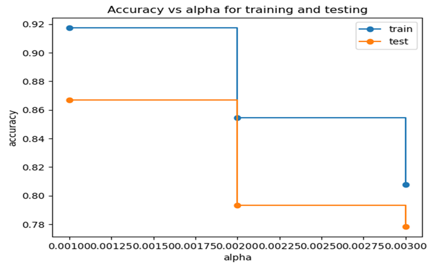
Figure 1: Training and Testing Accuracies
The Decision Tree Algorithm, specifically the Decision Tree Classifier, is a machine learning technique devised to address classification challenges. It belongs to the decision tree family of algorithms, which are widely employed in supervised learning tasks. This algorithm operates by constructing a hierarchical, tree-like structure in which each node corresponds to a decision based on multiple attribute values. The algorithm is as follows;
Based on the decision tree diagram, the health status of pregnant women can be classified into three categories: ‘high’, ‘low’ and ‘mid’ risk. The tree starts with a condition on age; there are three branches leading from this node each representing different conditions based on the women’s age. Depending on the initial classification by age, further classifications are made based on other vital signs like systolic blood pressure and body temperature. Here is the decision tree algorithm based on the averages:
Starting with Age:
If Age <= 29.5, go to Systolic blood pressure.
If Systolic blood pressure <= 125, go to body temp.
If Body temp <= 99, classify as mid risk,
Else if Body temp > 99, classify as high risk,
Else if Systolic blood pressure > 125, classify as high risk,
Else if Age >= 29.5 and <= 31.5, classify as mid risk,
Else if Age >31.5 and Blood sugar <= 7.95 classify as mid risk,
Else if Age > 31.5 and Blood sugar > 7.95 go to Systolic blood pressure
If Systolic blood pressure <= 133, classify as low risk,
Else if Systolic blood pressure >= 133, classify as high risk or other conditions here, return risk level.
The ultimate decision is determined by traversing the tree from the root node to a leaf node. The initial step in the Decision Tree Classifier involves selecting the feature that provides the highest information gain. Information gain quantifies how much a feature contributes to reducing uncertainty about the target variable, in this case, the risk level of pregnant women’s health.
This chosen feature serves as the starting point for constructing the tree, and data is partitioned based on its attribute values. The partitioning process is iteratively repeated until a predefined stopping condition is met, such as a specified threshold for the number of samples in each node or reaching the maximum tree depth. Figure 2 in the accompanying diagram illustrates the algorithm’s decision-making process and the interplay between features and the target variable. Notably, this algorithm can handle both continuous and categorical data, rendering it suitable for managing large dataset.
The root node, representing “Blood Sugar (BS),” was chosen with a value less than or equal to 7.93 mmol/L and an entropy value of 1.563. This selection was based on the highest information gain determined using the Gini index, a metric assessing the dataset’s impurity. The primary goal of constructing a decision tree is to partition the data into groups with low Gini indices, thereby enhancing our comprehension of the relationships between different classes and facilitating more informed decision-making.
Initially, the dataset for pregnant women consists of 679 samples. Based on their blood sugar levels, 178 individuals were categorized as having a mid-risk level, 275 as having a high-risk level, and 226 as having a low-risk level. Subsequent divisions were made based on variables such as systolic blood pressure and body temperature, with decisions ultimately determined by the majority representation in the leaf node.
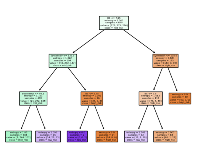
Figure 2 Decision Tree
Accuracy: The decision tree model achieved an accuracy of 0.8669 on the test data. This implies that the model correctly predicted the health risk level for approximately 86.69% of the samples in the test dataset.
Table 3: Classification Report for Decision Tree
| Precision | Recall | F1-score | Support | |
| High-risk | 0.87 | 0.85 | 0.86 | 47 |
| Low-risk | 0.86 | 0.78 | 0.82 | 80 |
| Mid-risk | 0.75 | 0.84 | 0.80 | 76 |
| Accuracy | 0.82 | 203 | ||
| Macro avg | 0.83 | 0.82 | 0.82 | 203 |
| Weighted avg | 0.82 | 0.82 | 0.82 | 203 |
Table 3 above shows the classification report realized when the dataset from health status of women were analysed and precision measures the accuracy of the positive predictions made by the model.
Precision and Recall:
For ‘high risk’ class, the precision is high (0.87) as well as the recall (0.85) indicating that a significant portion of women with ‘high risk’ health status was correctly identified with relatively few false positives.
For ‘low risk’ class, the model has a high precision (0.86) and high recall (0.78). This suggests that the model correctly identifies many ‘low risk’ cases when it predicts ‘low risk’ with very few false positives.
For ‘mid risk’ class, the model has a high precision (0.75) and high recall (0.84). this indicates that a significant portion of the women with ‘mid risk’ health status was identified correctly with very few false positives.
F1-Score:
The F1-score provides a balance between precision and recall. All the categories (class) have reasonably high F1-scores (0.86, 0.82 and 0.80 respectively). This means that the balance between precision and recall for all classes are relatively strong.
The macro average measuring the unweighted mean of precision, recall and F1-score are (0.83, 0.82 and 0.82 respectively) provides an overall view of how the model performed without considering class imbalances. The weighted average takes into account class imbalances by weighting the metrics by the number of samples in each class and the values are (0.82, 0.82 and 0.82 respectively) for precision, recall and F1-score.
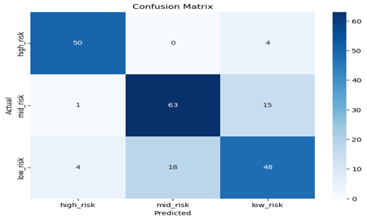
Figure 3: Confusion Matrix for Decision Tree
The numbers in the confusion matrix represent the number of instances that fall into each category with the rows representing the actual values, and the columns representing the predicted values. The matrix is labelled with “high_risk”, “low_risk”, and “mid_risk” on both of the axis.
The confusion matrix is used to evaluate how well a classification model is performing by comparing the predicted class labels with the actual class labels of a dataset. The values 50, 63 and 48 of the pregnant women with high_risk level, mid_risk level and low_risk level respectively is well classified because the class that is predicted actually occurred. Other values in all the rows and columns are represented as follows;
The first row of the confusion matrix represents the instances where the actual value was “high_risk”. The numbers in the first row are as follows:
50: This is the number of instances where the actual value was “high_risk” and the predicted value was also “high_risk”. This is a true positive (TP) case, meaning the model correctly predicted the presence of the health condition.
0: This is the number of instances where the actual value was “high_risk” but the predicted value was “mid_risk”. This is a false negative (FN) case, meaning the model incorrectly predicted the absence of the health condition.
4: This is the number of instances where the actual value was “high_risk” but the predicted value was “low_risk”. This is another false negative (FN) case, meaning the model incorrectly predicted the absence of the health condition.
The second row of the confusion matrix represents the instances where the actual value was “mid_risk”. The numbers in the second row are as follows:
63: This is the number of instances where the actual value was “mid_risk” and the predicted value was also “mid_risk”. This is a true negative (TN) case, meaning the model correctly predicted the absence of the health condition.
1: This is the number of instances where the actual value was “mid_risk” but the predicted value was “high_risk”. This is a false positive (FP) case, meaning the model incorrectly predicted the presence of the health condition.
15: This is the number of instances where the actual value was “mid_risk” but the predicted value was “low_risk”. This is another false negative (FN) case, meaning the model incorrectly predicted the absence of the health condition.
The third row of the confusion matrix represents the instances where the actual value was “low_risk”. The numbers in the third row are as follows:
4: This is the number of instances where the actual value was “low_risk” and the predicted value was “high_risk”. This is a false positive (FP) case, meaning the model incorrectly predicted the presence of the health condition.
48: This is the number of instances where the actual value was “low_risk” and the predicted value was also “low_risk”. This is a true negative (TN) case, meaning the model correctly predicted the absence of the health condition.
18: This is the number of instances where the actual value was “low_risk” but the predicted value was “mid_risk”. This is false positive (FP) case, meaning the model incorrectly predicted the presence of the health condition.
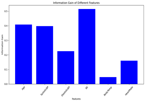
Figure 4: Information gain of the features
From the decision tree, the column BS (Blood sugar) has higher information gain, followed by age and Systolic blood pressure. There, it has more importance in the predicting the health status of the pregnant women. The measure of feature importance in Decision tree is achieve by calculating the information gain of each feature column. The higher the information gain of a feature column, the higher the purity.
Logistic Regression
Logistic regression is a supervised machine learning model that predicts data by using a linear relationship between each feature column and the target column. In logistic regression a linear line (mc + b) will be used to predict each class, where “m” is the coefficient of the x-axes (c) and “b” are the slope and intercept of the regression line. So, since we have three classes, each feature column will have three-line equations, one for each class in that column feature column. The line equation for each value of the feature column, i.e “c” with the highest probability will be the predicted class. In logistic regression, a supervised machine learning model, we aim to predict the health risk level of pregnant women (classified as high_level, mild_level, and low_level) based on various vital signs (age, systolic blood pressure, diastolic blood pressure, blood sugar, body temperature, and heart rate). Below are the results of the coefficient of logistic regression obtained using machine learning:
Coefficients for each class: For each of the three health risk classes (‘high_risk,’ ‘low_risk,’ and ‘mild_risk’), there are corresponding coefficients that indicate the importance of each feature in predicting that specific class
Class ‘high_risk’: [-0.08636582 0.31792099 0.42667279 1.17148158 0.49599125 0.28280912]
Class ‘low_risk’: [ 0.07887354 -0.69133654 0.03583753 -1.1496478 -0.52362363 -0.20292175]
Class ‘mid_risk’: [ 0.00749228 0.37341555 -0.46251031 -0.02183378 0.02763238 -0.07988737]
Here are the interpretations of the results:
The importance of each feature in predicting the different health risk classes can be analyzed using the coefficients obtained from the logistic regression model. For Class high risk, the coefficient of Age is (-0.08636582), Systolic Blood Pressure (0.31792099), Diastolic Blood Pressure (0.42667279), Blood Sugar(1.17148158), Body Temperature(0.49599125) and Heart Rate has value (0.28280912).
For Class low risk, the coefficient of Age is (0.0788735), Systolic Blood Pressure (-0.69133654), Diastolic Blood Pressure (0.03583753), Blood Sugar (-1.1496478), Body Temperature(-0.52362363) and Heart Rate has value (-0.20292175). For class mid risk, Age is (0.00749228), Systolic Blood Pressure (0.37341555), Diastolic Blood Pressure (-0.46251031), Blood Sugar (-0.02183378), Body Temperature (0.02763238) and Heart Rate (-0.07988737)
These coefficients indicate the direction and magnitude of the impact of each vital sign on the likelihood of a specific health risk level. For example, in ‘high_risk’ predictions, blood sugar and Systolic blood pressure have positive coefficients, suggesting they may contribute to a higher risk level, while in ‘low_risk’ predictions, these same features have negative coefficients, indicating they may contribute to a lower risk level.
Accuracy: The logistic regression model achieved an accuracy of 0.6256 on the test data. This means that the model correctly predicted the health risk level for approximately 62.562% of the samples in the test dataset.
Table 4: Classification Report for Logistic Regression
| Precision | Recall | F1-score | Support | |
| High-risk | 0.70 | 0.85 | 0.77 | 47 |
| Low-risk | 0.62 | 0.89 | 0.73 | 80 |
| Mid-risk | 0.68 | 0.28 | 0.39 | 76 |
| Accuracy | 0.65 | 203 | ||
| Macro avg | 0.67 | 0.67 | 0.63 | 203 |
| Weighted avg | 0.66 | 0.65 | 0.61 | 203 |
Table 4.3 above show the classification report obtained when the dataset from the health status of women were analysed.
Precision and Recall:
Precision measures the accuracy of the positive predictions made by the model.
For ‘high_risk’, the precision is 0.70. Out of all instances predicted as ‘high_risk’, 70% were correct. For ‘low_risk’, the precision is 0.62. Out of all instances predicted as ‘low_risk’, 62% were correct. For ‘mid_risk’, the precision is 0.68. Out of all instances predicted as ‘mid_risk’, 68% were correct.
Recall, also known as sensitivity or true positive rate, measures the ability of the model to identify all the positive instances. For ‘high_risk’, the recall is 0.85. The model correctly identifies 85% of the actual ‘high_risk’ instances. For ‘low_risk’, the recall is 0.89. The model correctly identifies 89% of the actual ‘low_risk’ instances. For ‘mid_risk’, the recall is 0.28. The model correctly identifies only 28% of the actual ‘mid_risk’ instances.
F1-Score:
The F1-score is the harmonic mean of precision and recall and provides a balance between the two. For ‘high_risk’, the F1-score is 0.77, indicating a balance between precision and recall for ‘high_risk’. For ‘low_risk’, the F1-score is 0.73, indicating a balance between precision and recall for ‘low_risk’. For ‘mid_risk’, the F1-score is 0.39, suggesting that the model struggles to balance precision and recall for ‘mid_risk’. However, the ‘support’ column shows the number of samples in each class.
The macro average is the unweighted mean of precision, recall, and F1-score across all classes. In this case, it’s about 0.67, 0.67, and 0.63, respectively. This provides an overall view of how the model performs without considering class imbalances, while the weighted average takes into account class imbalances by weighting the metrics by the number of samples in each class. The weighted average precision, recall, and F1-score are approximately 0.66, 0.65, and 0.61, respectively.
Visualization of the feature Importance Using Logistic Regression: The bar plot in figure 5 below displays the feature importance of selected vital signs based on the logistic regression approach. In terms of feature importance, body temperature is the most influential factor, followed by blood sugar, while age has a negative influence.
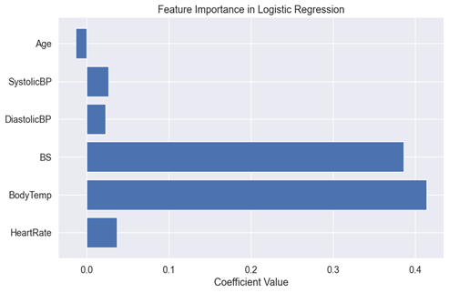
Figure. 5: The feature Importance Using Logistic Regression
Body temperature is the most important feature when determining the health status of pregnant women. A higher body temperature is associated with a higher risk of health issues, which is why it carries significant weight in the model. The second most important feature is blood sugar. Elevated blood sugar can be an indicator of health problems, making it an essential factor in health status prediction. Surprisingly, age has a negative influence, as indicated by the negative bar. This implies that, in this specific model, older age is associated with a lower health risk, which might seem counter-intuitive.
These feature importance are based on the logistic regression model’s coefficients. The model has learned from the data that body temperature and blood sugar are strong indicators of health status, while age plays a less influential role.
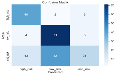
Figure 6: Confusion Matrix for Logistic Regression
The numbers in the confusion matrix represent the number of instances that fall into each category. The rows represent the actual values, while the columns represent the predicted values. The matrix is labelled with “high_risk”, “low_risk”, and “mid_risk” on both the x and y axis. The numbers in each cell represent the number of instances that fall into each category. For example, if we look at the cell in the first row and first column, it tells us that there were 40 instances where the actual value was “high_risk” and the predicted value was also “high_risk” also cell in the third row and second column tells us that there were 42 instances where the predicted value “low_risk” and the actual value was “mid_risk’. Similarly, if we look at the cell in the second row and third column, it tells us that there were 5 instances where the actual value was “low_risk” but the predicted value was “mid_risk”. The confusion matrix is used to evaluate how well a classification model is performing by comparing the predicted class labels with the actual class labels of a dataset.
The first row of the confusion matrix represents the instances where the actual value was “high_risk”. The numbers in the first row are as follows:
40: This is the number of instances where the actual value was “high_risk” and the predicted value was also “high_risk”. This is a true positive (TP) case, meaning the model correctly predicted the presence of the health condition.
2: This is the number of instances where the actual value was “high_risk” but the predicted value was “low_risk”. This is a false negative (FN) case, meaning the model incorrectly predicted the absence of the health condition.
5: This is the number of instances where the actual value was “high_risk” but the predicted value was “mid_risk”. This is another false negative (FN) case, meaning the model incorrectly predicted the absence of the health condition.
The second row of the confusion matrix represents the instances where the actual value was “low_risk”. The numbers in the second row are as follows:
71: This is the number of instances where the actual value was “low_risk” and the predicted value was also “low_risk”. This is a true negative (TN) case, meaning the model correctly predicted the absence of the health condition.
4: This is the number of instances where the actual value was “low_risk” but the predicted value was “high_risk”. This is a false positive (FP) case, meaning the model incorrectly predicted the presence of the health condition.
5: This is the number of instances where the actual value was “low_risk” but the predicted value was “mid_risk”. This is another false positive (FP) case, meaning the model incorrectly predicted the presence of the health condition.
The third row of the confusion matrix represents the instances where the actual value was “mid_risk”. The numbers in the third row are as follows:
13: This is the number of instances where the actual value was “mid_risk” and the predicted value was “high_risk”. This is a false positive (FP) case, meaning the model incorrectly predicted the presence of the health condition.
21: This is the number of instances where the actual value was “mid_risk” and the predicted value was also “mid_risk”. This is a true positive (TP) case, meaning the model correctly predicted the presence of the health condition.
42: This is the number of instances where the actual value was “mid_risk” but the predicted value was “low_risk”. This is false negative (FN) case, meaning the model incorrectly predicted the absence of the health condition.
Support Vector Machine (SVM)
Just like the logistic regression model, in SVM each column will also have three sets of line equation. So the feature importance is a measure of the coefficient of each class. Figures 3, 4 and 5 show the feature importance using the support vector machine model.
Table 5: Classification Report for SVM:
| Precision | Recall | F1-score | Support | |
| Low-risk | 0.60 | 0.88 | 0.71 | 80 |
| Mid-risk | 0.74 | 0.30 | 0.43 | 76 |
| High-risk | 0.71 | 0.85 | 0.78 | 47 |
| Accuracy | 0.66 | 203 | ||
| Macro avg | 0.69 | 0.68 | 0.64 | 203 |
| Weighted avg | 0.68 | 0.66 | 0.62 | 203 |
Table 5 shows the classification report obtained when the dataset from the health status of women were analysed using the Support Vector Machine (SVM) model.
Accuracy: The overall accuracy of the model is 0.6552, indicating that the model correctly predicts the health status category for approximately 65.52% of the pregnant women in the test dataset.
Precision and Recall:
For the low risk category, the model has a high precision (0.60) and a high recall (0.88), indicating that it correctly identifies a significant portion of women with ‘low risk’ health status and has relatively few false positives.
For the mid risk category, the precision is relatively high (0.74), but the recall is low (0.30). This suggests that the model correctly identifies many mid risk cases when it predicts mid risk, but it misses a substantial number of mid risk cases.
For the high risk category, the model has a high precision (0.71) and a high recall (0.85), indicating it correctly identifies a substantial portion of women with high risk health status with relatively few false positives.
F1-Score: The F1-scores provide a balance between precision and recall. While the low risk and high risk categories have reasonably high F1-scores (0.71 and 0.78, respectively), the mid risk category has a lower F1-score (0.43). This suggests that the model’s performance for mid risk cases is weaker compared to the other categories.
In summary, based on these results, you can conclude the following for SVM:
– The model is relatively successful in identifying women with ‘low risk’ and ‘high risk’ health status, with good precision and recall for these categories.
– The model faces challenges in correctly identifying women with ‘mid risk’ health status, with lower recall and F1-score for this category. This may indicate that the model struggles to distinguish between ‘mid risk’ and other health status categories.
The macro average is the unweighted mean of precision, recall, and F1-score across all classes. In this case, it’s about 0.69, 0.68, and 0.64, respectively. This provides an overall view of how the model performs without considering class imbalances. The weighted average takes into account class imbalances by weighting the metrics by the number of samples in each class. The weighted average precision, recall, and F1-score are approximately 0.68, 0.66, and 0.62, respectively.
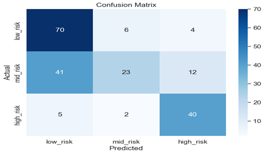
Figure 6: Confusion Matrix for Support Vector Machine
The confusion matrix shows that 70 of the pregnant women with low risk health are classified well, 23 of mid risk level and 40 of the high risk level are classified well respectively.
Using the support vector machine, the first row of the confusion matrix represents the instances where the actual value was “low_risk”. The numbers in the first row are as follows:
70: This is the number of instances where the actual value was “low_risk” and the predicted value was also “low_risk”. This is a true negative (TN) case, meaning the model correctly predicted the absence of the health condition.
6: This is the number of instances where the actual value was “low_risk” but the predicted value was “mid_risk”. This is a false positive (FP) case, meaning the model incorrectly predicted the presence of the health condition.
4: This is the number of instances where the actual value was “low_risk” but the predicted value was “high_risk”. This is another false positive (FP) case, meaning the model incorrectly predicted the presence of the health condition.
The second row of the confusion matrix represents the instances where the actual value was “mid_risk”. The numbers in the second row are as follows:
23: This is the number of instances where the actual value was “mid_risk” and the predicted value was also “mid_risk”. This is a true positive (TP) case, meaning the model correctly predicted the presence of the health condition.
12: This is the number of instances where the actual value was “mid_risk” but the predicted value was “high_risk”. This is a false positive (FP) case, meaning the model incorrectly predicted the presence of the health condition.
41: This is the number of instances where the actual value was “mid_risk” but the predicted value was “low_risk”. This is false negative (FN) case, meaning the model incorrectly predicted the absence of the health condition.
The third row of the confusion matrix represents the instances where the actual value was “high_risk”. The numbers in the third row are as follows:
2: This is the number of instances where the actual value was “high_risk” and the predicted value was “mid_risk”. This is a false negative (FN) case, meaning the model incorrectly predicted the absence of the health condition.
40: This is the number of instances where the actual value was “high_risk” and the predicted value was also “high_risk”. This is a true positive (TP) case, meaning the model correctly predicted the presence of the health condition.
5: This is the number of instances where the actual value was “high_risk” but the predicted value was “low_risk”. This is another false negative (FN) case, meaning the model incorrectly predicted the absence of the health condition
Comparison of Models Base on Accuracy
| Table 4.5: Model Accuracy | |||
| Model | Decision tree | Logistic Regression | SVM |
| Accuracy | 0.866995 | 0.625616 | 0.655203 |
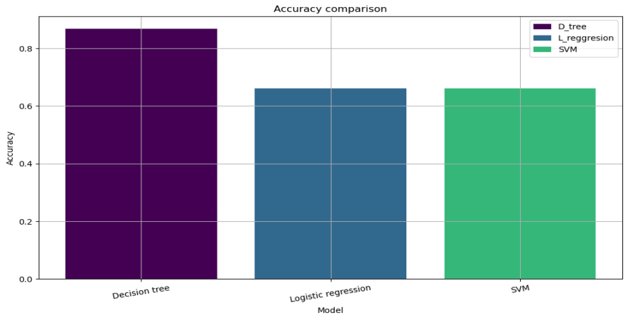
Figure 6: Model Comparison Based on Accuracy Values Using Barchart
Based on the barchart in figure 6, the decision tree model has the highest accuracy value of 0.866995, followed by SVM with an accuracy value of 0.655203 and logistic regression with an accuracy value of 0.625616. This means that the decision tree model is the most accurate model in predicting the health status of pregnant women, followed by SVM and logistic regression. The accuracy values are a measure of how well the models performed in predicting the health status of pregnant women. The higher the accuracy value, the better the model performed. In conclusion, using the available dataset, decision tree model is best for predicting health status of the pregnant women since it has the highest accuracy value.
SUMMARY AND CONCLUSION
Three models were assessed for predicting the impact of vital signs on health risk of pregnant mothers: Decision Tree, Multiple logistic Regression and Support Vector Machine (SVM). The evaluation of model performance was done using metrics such as Precision, Accuracy, F1-score and Recall (sensitivity). The results revealed that the Decision tree model achieved the highest accuracy of 0.8669 (86.69%), that indicates correct prediction in 86.69% of the cases. Also, it achieved the highest precision for all the risk categories (high_risk, low_risk and mid_risk) with values (87%, 86% and 75% respectively) implying lower likelihood of false positive predictions for all risk categories. The Logistic Regression model achieved an accuracy of 0.6256, indicating correct prediction in 62.56% of the cases. It exhibited a high recall (sensitivity) for the high_risk and low_risk categories (85% and 89%) but mid_risk has low recall with 28% indicating the model correctly identifies few of the actual mid_risk cases. The SVM model achieved an accuracy of 0.6552, this indicates correct prediction in 65.52% of the cases. The F1-score for (high, low and mid) risk categories are 78%, 71% and 43% implying that high_risk and low_risk have reasonably high balance between precision and recall and mid_risk is weak.
Generally, the SVM model is relatively successful in identifying pregnant women with low_risk and high_risk health status with good precision and recall (sensitivity) but faces challenge in identifying pregnant women with mid_risk health status with lower recall (sensitivity) and F1-score. This may indicate that the model struggles to distinguish between mid_risk and other category of health status. Also, the Decision Tree model is successful in identifying pregnant women in high_risk, low_risk and mid_risk health status with good precision and recall (sensitivity) for these categories. The F1-scores are also high indicating the model did not struggle to distinguish between the categories of health status. Similarly, the Logistic Regression model is relatively successful in identifying pregnant women with high_risk and low_risk health status with good precision and recall (sensitivity) for both categories. The mid_risk has low recall (sensitivity) and F1-score indicating that it struggles to identify and distinguish mid_risk and other health status categories.
This makes the Decision Tree model more reliable for classification task. The choice of the “best” model depends on specific requirements and priorities with Decision Tree being preferred for correctly achieving good accuracy, precision, recall and F1-score.
In conclusion, the Decision Tree model appears to be a promising approach for predicting the impact of vital signs on health risk of pregnant mothers. It exhibited high precision, high recall (sensitivity) and a balanced F1-score, suggesting accurate predictions with very low rate of false positives.
REFERENCES
- Abe Shigeo (2005). Support Vector Machines for Pattern Classification. Springer
- Macrohon, J. Jerison E., Charlyn Nayve Villavicencio, Xavier Alphonse Inbaraj & J. H. Jeng (2022) A Semi-Supervised Machine Learning Approach in Predicting High-Risk Pregnancies in the Philippines.” Diagnostics 12.
- Marques Lobo & João Alexandre (2021)., IoT-Based Smart Health System for Ambulatory Maternal and Fetal Monitoring, in IEEE Internet of Things Journal, 8, (23), pp 16814-16824, doi: 10.1109/JIOT.2020.3037759.
- Martine De Cock, Rafael Dowsley, Caleb Horst, Raj Katti, Anderson C. A. Nascimento, Wing-Sea Poon & Stacey Truex (2019). Efficient and Private Scoring of Decision Trees, Support Vector Machines and Logistic Regression Models based on Pre-Computation, in IEEE Transactions on Dependable and Secure Computing, 16(2), pp. 217-230, 1 March-April 2019, doi: 10.1109/TDSC.2017.2679189
- Matthew M. Churpek, Richa Adhikari, & Dana P. Edelson, (2016) The value of vital sign trends for detecting clinical deterioration on the wards, Resuscitation, 102, pp 1-5, ISSN 0300-9572, https://doi.org/10.1016/j.resuscitation.2016.02.005
- Mennickent D, Rodr´ıguez A, Opazo MC, Riedel CA, Castro E, Eriz-Salinas A, Appel-Rubio J, Aguayo C, Damiano AE, Guzma´ n-Gutierrez E & Araya J (2023), Machine Learning Applied in Maternal and Fetal Health: A narrative review focused on pregnancy diseases and complications. Front. Endocrinol. 14(11) pp 30-39
- Mohd Javaid, Abid Haleem, Ravi Pratap Singh, Rajiv Suman & Shanay Rab, (2022) Significance Of Machine Learning in Healthcare: Features, Pillars and Applications’’ International Journal of Intelligent Networks, 3, Pp 58-73,ISSN 2666-6030, https://doi.org/10.1016/j.ijin.2022.05.002
- Ngiam KY & Khor IW. (2019) Big data and machine learning algorithms for health-care delivery. Lancet Oncol. 20(5):e262-e273. doi: 10.1016/S1470-2045(19)30149-4. Erratum in: Lancet Oncol. 2019 Jun;20(6):293. PMID: 31044724.
- Rescinito, Riccardo, Matteo Ratti, Anil Babu Payedimarri & Massimiliano Panella (2023) Prediction Models for Intrauterine Growth Restriction Using Artificial Intelligence and Machine Learning: A Systematic Review and Meta-Analysis, Healthcare 11
- Seth Flam (2023) Machine Learning in Healthcare – Benefits & Use Cases (foreseemed.com)
- Vousden, N., Nathan, H.L. & Shennan, A.H. (2018) Innovations in vital signs measurement for the detection of hypertension and shock in pregnancy. Reprod Health 15 (Suppl 1), 92 . https://doi.org/10.1186/s12978-018-0533-4