Mathematical Model for the Determination of Optimal Salary in Defined Benefit Pension Plan with Early Retirement, An Application of Smooth-Pasting Condition
- Matthew O. Adaji
- 128-144
- Oct 14, 2023
- Mathematics
Mathematical Model for the Determination of Optimal Salary in Defined Benefit Pension Plan with Early Retirement, An Application of Smooth-Pasting Condition
Matthew O. Adaji
Department of Mathematics/Statistics, School of Technology, Benue State Polytechnic, Ugbokolo. Nigeria
DOI: https://doi.org/10.51584/IJRIAS.2023.8915
Received: 26 August 2023; Revised: 08 September 2023; Accepted: 13 September 2023; Published: 14 October 2023
Abstract
The paper seeks to apply the mathematical model formulated by Adaji, et al (2015) to determine the optimal financial value of the retirement benefit Sf by applying Smooth Pasting condition. We examined the smooth pasting condition (tangency condition) along the optimal point at the boundary for an American put by considering the gradient, ∂V/∂S more closely and found that as long as V(S) coincides with the straight line, K-S gradient equals-1. We used Microsoft excel spread sheet facility to perform the individual computation for the last 25 years of service for University Senior Lecturers and the last 10 years of service for University Professors. The optimal salary Sf was determined by drawing a vertical line from the tangent perpendicularly to the horizontal axis (salary axis). We recommend the applictaion of this model to individuals as well as cooperate organisations so as maximise the expected retirement benefit. Early retirement alternate should be encouraged so that the teeming population of unemployed youths can take up the vacancies created as a result of early retirement.
Keyword: Smooth Pasting, Optimal Stopping, Value Function and Gain Function
I. Introduction
There comes a time in our lives when we as employees consider starting a pension plan – either on the advice of a friend, a relative, on our own volition or by law. The choice of plan may depend on various factors, such as the age and salary of the individual, number of years of expected employment, as well as options to retire early or late.
Calvo-Garrido and Vazquez (2012) presented a partial differential equation (PDE) model governing the value of a defined pension plan without the option for early retirement. They say that it is important to develop mathematical models to compute the value of this liability in order to estimate the financial situation of the institution or company that has the obligation with the member of pension plan.
Calvo-Garridoand Vazquez (2012) proposed future work concerning the possibility of early retirement. According to them, linear complementarity formulations of the resulting variational inequality can be analyzed to obtain the existence of solutions, and suitable numerical methods are required to obtain the pension plan value.
American options are financial derivatives that can be exercised at any time before maturity, in contrast to European options which have fixed maturities. The prices of American options are evaluated as an optimization problem, in which one has to find the optimal time to exercise in order to maximize the claim option payoff. The smooth pasting property (condition), states that the value function must be continuously differentiable everywhere, and yields conditions, which uniquely determine the optimal stopping region. Art of smooth pasting includes a heuristic justification for the differentiability of value functions at optimal stopping thresholds. In pure stopping problems, “smoothness” requires (and means) that the value functionsis once differentiable, and is known as the smooth pasting condition.
II. Literature Review
III. Assumptions of the Model
-
The model satisfies smooth pasting condition
-
A member of the plan would retire when he/she maximizes the benefits of retirement among all possible dates (stopping times) to retire.
-
Optimal stopping problem with a value function V(St)=supτ≤T Es e-τr Vτ (K-St) satisfies geometric Brownian motion, dSt = μSt dt+ σSt dWt
-
The infinitesimal generator of the (strong) Markov process S is given by Ls V=rS ∂/∂S+σ2/2 S2 ∂2/(∂S2 ).Standard Markovian arguments suggest that V from assumption (g) solves the following free boundary problem of parabolic type Ls V=rV
3.1 Parameters and Variables of the Model
The following parameters (functions) and variables are used in this research work:
V=V(S,t )=V(St )is the financial value of retirement benefit in the time interval 0<t≤T;
S=St = salary at time, t;
Sf = Optimal salary;
K= strike salary;
S-K = Payoff for the call option (American call option for a fixed K and any given salary, S) representing an employer’s option
K-S= Payoff for the put option (American put option for a fixed K and any given salary,S) representing an employee’s option
(S-K)+=maxs (S-K,0) assumed to occur at the optimal boundary (call option)
(K-S)+=mins (K-S,0) assumed to occur at the optimal boundary (put option)
V(Sf )= Optimal financial value of retirement benefit (is also the same as the optimal retirement benefits) with respect to salary
t= Time (in year) spent with the pension plan
r=the salary growth rate or Accrual rate
μ=(r-δ) is the expected return of the salary (asset)
δ=annual dividend yield δ≥0 of the asset (salary) (when δ=0,then μ=r)
σ= The volatility of the salary (also the standard deviation)
T =Worker’s expected retirement time (maturity or expiry time) in years
τ= stopping time
τf= optimal stopping time
C, D= continuation set and stopping set respectively
Wt=geometric Brownian process, (Disturbance factor)
k1 ,k2= arbitrary constants,
w+, w–= respective positive and negative roots of an auxiliary equation
Rd=d-dimensional Euclidean space
Ls = infinitesimal operator of S
Vτ = value function at stopping time, τ,
Φτ = gain function at stopping time, τ,
ES=expectation with respect to S
(Ω,F,P)=probability space
Ft =filtration
Remark 1: The Shift Operator
The shift operator is useful in defining the (strong) Markov property.
The Measure PS
Let W=(Wt )t≥0 be a standard Brownian motion under the measure P. Thus each Wt is a random variable defined on a probability space (Ω,F,P), and W0=0 under P. Now define St= S+Wt, for all 0 ≤ t <∞. Then St is a random variable on the same probability space. Moreover, we see that S0= S under P.
Definition 1.
Let Ω be some space of functions from [0,∞]into R. The shift operator θt: Ω→Ω defined by (θt (ω) )(s) = ω(t+s)
for ωϵΩ (Typically, we regard ωϵΩ as a sample path of some stochastic process.) Suppose thatS=(S_t )_(t≥0) is a stochastic process on the probability space Ω,F,P the following useful results are given without proofs.
Definition 2.
If a process S=(St )t≥0 is equipped with the filtration (Ft )t≥0, with F=σ(⋃t≥0 Ft ), then S has the (strong) Markov property if any of the following
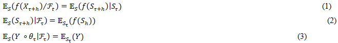
for all S, all stopping times τ, all h>0, any bounded Borel-measurable function f, and any (bounded) F-measurable random variable Y.
Remark 1:The (Strong) Markov Property
The future behaviour of a Markov process is not dependent on its past, but only on its current value.
Definition 3

It is important to note that for n=1 the above infinitesimal generator of the strong Markov process S becomes
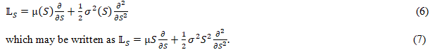
Remark 2: The Infinitesimal Generator
The infinitesimal generator enables us to associate a second order partial differential operator with a stochastic process.
Definition 4.
A function V is called superharmonic if ES (V(Sτ ))≤V(S) (8)
for all S, and for every stopping time τ. If the process S has the (strong) Markov property and is adequately regular, this is equivalent to saying that the process V(St)t≥0 is a supermartingaleunder Ps, for each S.
Remark 3:
Dynkin’superharmonic characterisation of the value function for Markov processes is captured in the four statements of the following theorem.
Theorem 1.
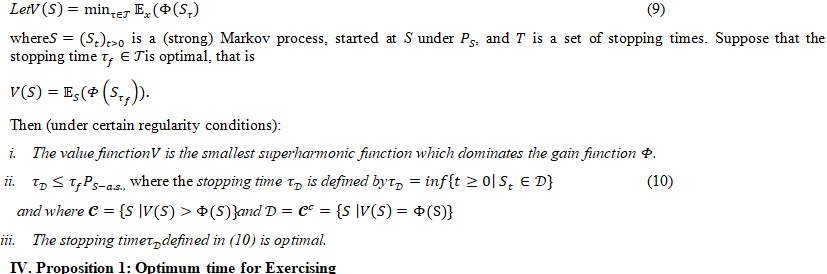
IV. Proposition 1: Optimum time for Exercising
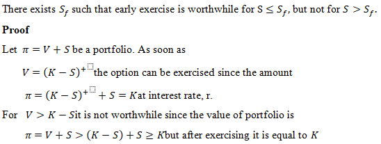
The value Sf depends on time, and it is termed the free boundary value. We have
V(S,t)=(K-S)+,^ S≤Sf (t)
V(S,t)> (K-S)>Sf (t)
Since the free-boundary value is not known, it must be determined with the option price.
For large S, the put option satisfies the Black – Scholes equation (Merton, 1973).
This is smooth pasting condition.
According to Merton (1973), American Put option can be determined by solving
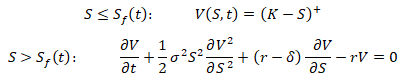
With the endpoint condition
V(S,T)=(K-S)
And the boundary conditions
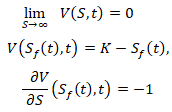
Our formulation follows perpetual American put option. Perpetual American put option has value function that is a function of the stock price, V=V(S) only and its optimal stopping boundary is a constant function.
So, the boundary conditions become
 (11)
(11)
Our formulation follows Perpetual (infinite) American put option. Perpetual American put option has value function that is a function of the stock price, V=V(S) only and its optimal stopping boundary is a constant function.
4.1 Derivation of the Solution by the Markovian Method
Adaji, et al (2015) formulated a mathematical model to determine the financial value of retirement benefit, V(S) (free arbitrage price or the option value) for perpetual American put. The study considers one pricing formulation of American options, namely, the optimal stopping formulation as equivalence of a free-boundary problem. The optimal stopping problem on perpetual American put was formulated and its solutions found. The solutions found were analysed systematically by applying matching value condition, smooth pasting condition, asset equilibrium condition and the boundary condition. They used the free-boundary approach to derive the solution. The model was based on final salary given by
 (12)
(12)
where K-S is the payoff in the case of American put option at any given value of salary, S.
The equation (12) is used to determine the financial value of retirement benefit, V(S) (free arbitrage price or the option value) for perpetual American put. It can only be determined if its optimal value, Sf is known. V(Sf )is the value of the pension benefit that is optimal to retire. Our task here (amongst other things) is to use (12) to determine the financial value of the retirement benefit Sf by applying Smooth Pasting condition amongst other financial formulations.
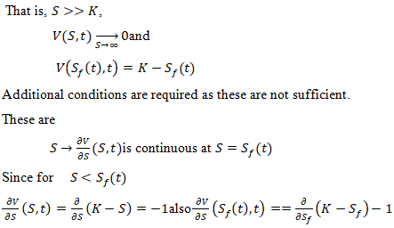
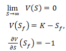
We would like to examine the smooth pasting condition (tangency condition) along the optimal point at boundary for an American put. At S=S_f, the value of the optimal point of American put is K-Sf. This is termed as the value matching condition:
V(Sf )=K-Sf (13)
Suppose Sf is a known continuous function, the pricing model becomes a boundary value problem with a time dependent boundary. However, in the American put option model, Sf is not known in advance. Rather, it must be determined as part of the solution.
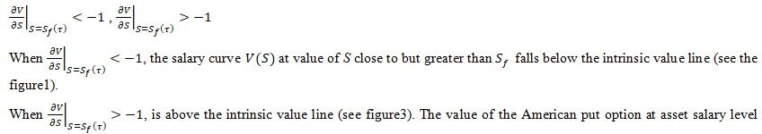
To be able to calculate the unknown boundary Sf, we need the smooth pasting condition, and therefore we consider the gradient, ∂V/∂S more closely. From our assumption that the model satisfies smooth pasting condition, it then implies that as long as V(S) coincides with the straight line, K-S with gradient equals -1 , and at the contact point, we will draw a vertical line from the tangent perpendicular to the horizontal axis to obtain Sf.
V. Results
The results obtained from computer programme of equations (12) in Chapter 3 are presented in Tables 1, 2, …, 6 and the corresponding graphs obtained from these tables are presented in Figures 1, 2, …, 6 to illustrate the performance of the model. For this purpose, the following model parameters are presented.
We show how the values are simulated using Excel package. The data we use in the computation are from Appendix B1.
We use Microsoft excel spread sheet facility to perform the individual computation for 25 years for University senior lecturers and 10 years for University Professors as shown in Tables 1 to 3.
This computation is applicable to various cadres of staff and institutions.
Substituting these parameters into the above programme, we have = POWER(Ai,-D1) *(1/D1) *POWER(D2/(1+D1),(D1+1))
where i = 1,2,3,…,25.
We compute financial values of retirement benefit for Senior lecturers in the last 25 years of service using simulation. For this category, we use
D1= 2r/σ2 =2(2.5)/12 =5;
D2=K=6020349;
S0=3091505
We use the process to compute financial value of retirement benefit for Professors in the last 10 years of service. For this category, we use
D1= 2r/σ2 =2(2.5)/12 =5;
D2=K=6020349;
S0=4580349.
Table 1:Data of Financial Value, V(S) of Retirement for University Senior Lecturers in the last 25 years of service when , K=6020349, S0=3091505, r=2.5, σ=1
| S | V=V(S) | V= (K-S) | X=0.5 |
| 3091505 | 158881.3024 | 2928844 | K=6020349 |
| 3216505 | 143892.1485 | 2803844 | |
| 3341505 | 130810.4339 | 2678844 | |
| 3466505 | 119335.0713 | 2553844 | |
| 3591505 | 109221.0848 | 2428844 | |
| 3716505 | 100267.6579 | 2303844 | |
| 3841505 | 92309.02575 | 2178844 | |
| 3966505 | 85207.46781 | 2053844 | |
| 4091505 | 78847.86872 | 1928844 | |
| 4216505 | 73133.46075 | 1803844 | |
| 4341505 | 67982.46543 | 1678844 | |
| 4466505 | 63325.42499 | 1553844 | |
| 4591505 | 59103.06732 | 1428844 | |
| 4716505 | 55264.58669 | 1303844 | |
| 4841505 | 51766.25086 | 1178844 | |
| 4966505 | 48570.26598 | 1053844 | |
| 5091505 | 45643.84668 | 928844 | |
| 5216505 | 42958.45013 | 803844 | |
| 5341505 | 40489.14222 | 678844 | |
| 5466505 | 38214.07047 | 553844 | |
| 5591505 | 36114.02384 | 428844 | |
| 5716505 | 34172.06353 | 303844 | |
| 5841505 | 32373.21208 | 178844 | |
| 5966505 | 30704.19051 | 53844 | |
| 6091505 | 29153.19528 | -71156 |
Table 2: Data of Financial Value, V(S) of Retirement for University Senior Lecturers in the last 25 years of service when, K=5491505, S0=3091505, r=2.5, σ=1
| S | V=V(S) | V=(K-S) | X=5 | |
| 1 | 3091505 | 722.7744 | 2928844 | K=5491505 |
| 2 | 3216505 | 592.8316 | 2803844 | |
| 3 | 3341505 | 489.9389 | 2678844 | |
| 4 | 3466505 | 407.7494 | 2553844 | |
| 5 | 3591505 | 341.5625 | 2428844 | |
| 6 | 3716505 | 287.8584 | 2303844 | |
| 7 | 3841505 | 243.9751 | 2178844 | |
| 8 | 3966505 | 207.8799 | 2053844 | |
| 9 | 4091505 | 178.0070 | 1928844 | |
| 10 | 4216505 | 153.1403 | 1803844 | |
| 11 | 4341505 | 132.3278 | 1678844 | |
| 12 | 4466505 | 114.8189 | 1553844 | |
| 13 | 4591505 | 100.0178 | 1428844 | |
| 14 | 4716505 | 87.44823 | 1303844 | |
| 15 | 4841505 | 76.72742 | 1178844 | |
| 16 | 4966505 | 67.54576 | 1053844 | |
| 17 | 5091505 | 59.65154 | 928844 | |
| 18 | 5216505 | 52.83897 | 803844 | |
| 19 | 5341505 | 46.93905 | 678844 | |
| 20 | 5466505 | 41.81227 | 553844 | |
| 21 | 5591505 | 37.34297 | 428844 | |
| 22 | 5716505 | 33.43486 | 303844 | |
| 23 | 5841505 | 30.00743 | 178844 | |
| 24 | 5966505 | 26.99308 | 53844 | |
| 25 | 6091505 | 24.33489 | -71156 |
Table 3: Data of Financial Value, V(S) of Retirement for University Senior Lecturers in the last 25 years of service when K=5000000, S0=3091505, r=2.5, σ=1
| S/NO | S | V=V(S) | V= (K-S) | X= 5 |
| 1 | 3091505 | 117295.1 | 2428844 | K=5520349 |
| 2 | 3216505 | 106229.3 | 2303844 | |
| 3 | 3341505 | 96571.60 | 2178844 | |
| 4 | 3466505 | 88099.84 | 2053844 | |
| 5 | 3591505 | 80633.13 | 1928844 | |
| 6 | 3716505 | 74023.21 | 1803844 | |
| 7 | 3841505 | 68147.70 | 1678844 | |
| 8 | 3966505 | 62904.93 | 1553844 | |
| 9 | 4091505 | 58209.92 | 1428844 | |
| 10 | 4216505 | 53991.22 | 1303844 | |
| 11 | 4341505 | 50188.47 | 1178844 | |
| 12 | 4466505 | 46750.38 | 1053844 | |
| 13 | 4591505 | 43633.20 | 928844 | |
| 14 | 4716505 | 40799.42 | 803844 | |
| 15 | 4841505 | 38216.75 | 678844 | |
| 16 | 4966505 | 35857.29 | 553844 | |
| 17 | 5091505 | 33696.85 | 428844 | |
| 18 | 5216505 | 31714.34 | 303844 | |
| 19 | 5341505 | 29891.36 | 178844 | |
| 20 | 5466505 | 28211.77 | 53844 | |
| 21 | 5591505 | 26661.40 | -71156 | |
| 22 | 5716505 | 25227.73 | -196156 | |
| 23 | 5841505 | 23899.72 | -321156 | |
| 24 | 5966505 | 22667.56 | -446156 | |
| 25 | 6091505 | 21522.52 | -571156 |
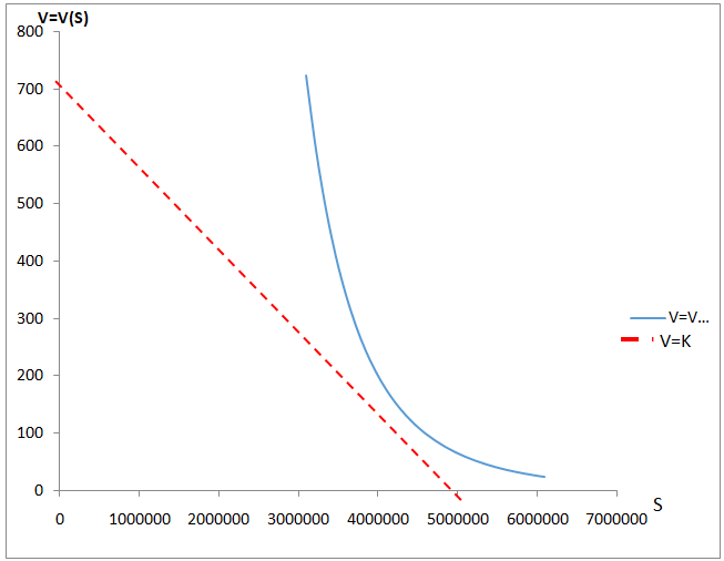
Figure 1:Graph of Financial Value, V(S) of Retirement for University Senior Lecturers in the last 25 years of service when K=6020349, S0=3091505, r=2.5, σ=1
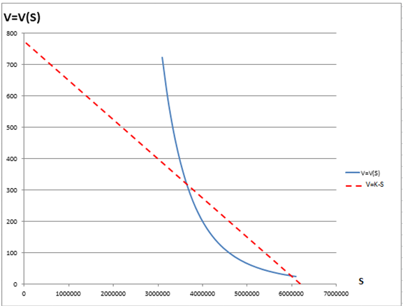
Figure 2:Graph of Financial Value, V(S) of Retirement for University Senior Lecturers in the last 25 years of service when K= N 5491505, S0=3091505, r=2.5, σ=1
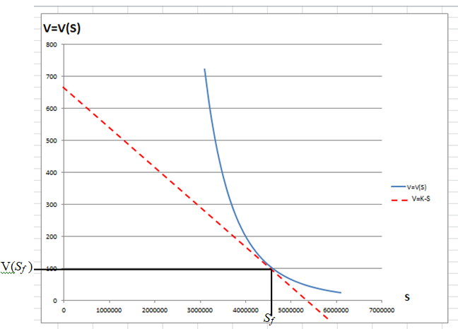
Figure 3:Graph of Financial Value, V(S) of Retirement for University Senior Lecturers in the last 25 years of service when K= 500000, S0=3091505, r=2.5, σ=1
VI. Discussion
In section 4, we validated the model by using empirical data from Consolidated University Salary Structure (CONUASS) to determine the optimal salary for early retirement for University Senior Lecturers in the last 25 years of service. Figures 1- 3 display the outputs of Tables 1-3 as we varied the values of K. We set K= N 6020349 in Figure 1, K= N 5491505 in Figure 2, K= N 5000000 and in Figure 3, K= N 6020349.
Figure1. The Figure displays the interaction of the salary curve and the straight line with negative slop. The line (K-S) cuts the curve, V=V(S) at two points. This means that we did not get the optimal point. This implies that the K= 6020349 is high and needed to be reduced.
Figure 2: It is a graph showing salary, S on the horizontal axis and financial value of retirement benefit V(S) of American put option on the vertical as for fixed strike salary, K=N5491505 per annum and the payoff, K-S of American put option for University Senior lecturers in the last 25 years of service. S0=3091505, 2r/σ2 =5. The value of the option meets the payoff function smoothly. The salary curve V(S) touches tangentially the intrinsic line at the point representing the value of the optimal retirement salary, Sf. The optimal value of the financial retirement benefit is got by drawing a vertical line from the tangent point to the horizontal line. The vertical line intercepts the salary axis at Sf= 4591505 per annum). The corresponding vertical axis V(Sf )=100.
Figure 3: This graph is showing salary, S and financial value of retirement benefit V(S) of American put option for fixed strike salary, K=N5000000 per annum and the payoff, K-S of American put option for University Senior lecturers in the last 25 years of service. S0=3091505,2r/σ2 =5. The Figure 3 displays the interaction of the salary curve and the straight line with negative slop. The line (K-S) and the curve, V=V(S) do not have contact at all. This means that we did not get the optimal point. This implies that the K=5000000 is low and needed to be increased.
The differences we observe in Figures 1 and 3, are direct consequences of varying K-S. We continue until we arrive at Figures 2 for the Senior Lecturers in the last 25 years of their service.
Figures 1 and 3 are not optimal while that of 2 is optimal for University Senior in the last 25 years of service.
VII. Conclusion and Recommendations
7.1 Conclusion
In the examples, we used Microsoft excel spread sheet facility to perform the individual computation for 25 years for University senior lecturers and 10 years for University Professors as shown in Tables 1 to 3.
We assumed that the smooth pasting condition holds, this assumption was used to find the optimal stopping region, and verified that this solution equals the optimal value function. This is what is referred to as “Art of Smooth Pasting,” which includes a heuristic justification for the differentiability of value functions at optimal stopping thresholds.
We demonstrated this by considering the behaviour of curve near Sf(τ). From our assumption that the model certifies smooth pasting condition, it then implies that as long as V(St) coincides with the straight line, K-S its gradient equals -1, and at the high contact point produces Sf (where (K-S)=(K-Sf)) we also have under the following two scenarios
close to Sf(τ) can be varied (increased by choosing a smaller value for Sf(τ). This explains why both cases do not correspond to the optimal exercise strategy.
In order to obtain optimality, we varied the value of (K-S) which represents a straight line. We continued until the line touched the curve tangentially as seen in figure 2.
The (K-S) reveals the relation between the strike salary, K (assumed to be greater than other salaries over the years). It has a negative slop which intercepts the salary axis (horizontal axis at K). The value of financial benefit (the vertical axis represents V(S) and the horizontal axis represents the salary axis.
The model is people-friendly in application as individual employee who does not have a mathematical background can also use it with ease. The application can be extended to every employee’s cadre. We also included the formula and the computation of gratuity in Tables 4 and 5.
7.2 Recommendations
We recommend the appliction of this model to individuals as well as cooperate organisations so as maximise the expected retirement benefit. This can only to achieved if we know the optmal point to retire.
We recommend that government at the federal, state and local level make public the salary growth rate as well as the strike salary of every cadre. Early retirement alternative should be encouraged so that the teeming population of unemployed youths can take up the vacancies created as a result of early retirement.
As was stated, this work is concerned with one dimension, however, it can be extended to higher dimensions. This is open to further research.
A computer programme could be developed to authomaticaly compute model equation (12) to determine the optimal salary instead of hearustic justification by the smooth pasting approach
Contributions: Investigation, Matthew Adaji; Writing – original draft, Matthew Adaji; Writing – review & editing, Matthew Adaji.
References
- Adaji, M. O, Onah, E. S, Kimbir, A. R, and Aboiyar, T (2015). Financial Valuation of Early Retirement Benefit in a Defined Benefit Pension Plan. International Journal of Mathematical Analysis and Optimization: Theory and Applications, [S.l.], pp. 67 – 82, Available at: <http://ijmao.unilag.edu.ng/article/view/286/158>.
- Bensoussan, A. (1984). On the theory of option pricing. Acta Appl. Math., 2: 139-158.
- Calvo-Garrido, M. C. and Vázquez, C. (2012). Pricing Pension plans based on average salary without early retirement: Partial differential equation modelling and numerical solution. The Journal of Computational Finance 16(1):111-140
- Guo, X and Shepp, L A (2001). Some optimal stopping problems with nontrivial boundaries for pricing exotic options J. Appl. Probab., 38 (3), pp. 647-658
- Hu, Y., Liang, G. and Tang, S., (2018) Exponential utility maximization and indifference valuation with unbounded payoffs. arXiv: 1707.00199v3,
- Karatzas, I. (1988). On the pricing of American options.Applied Mathematics and Optimization, 17:37-60.
- McKean, H. P. (1965). Appendix: A free boundary problem for the heat equation arising from a problem in mathematical economics. Industrial Management Review, 6:32-39.
- Mikhalevich, S. (1958). A Bayes test of two hypotheses concerning the mean of a normal process. VisnikKiiv. Univ.No. 1 (Ukrainian) (101-104).
- Oksendai, B (2000) Stochastic Differential Equations: An introduction with Applications. Springer.Seydel, Rüdiger. Tools for Computational Finance. pp. 143–145. ISBN3-540-40604-2.
- Shreve, E. S (2004). “Stochastic Calculus for Finance I, the Binomial Asset Pricing Model”. Carnegie Mellon University, USA.
- Sun, D, (2021) The Convergence Rate from Discrete to Continuous Optimal Investment Stopping Problem. Chin. Ann. Math. Ser. B 42, 259–280 https://doi.org/10.1007/s11401-021-0256-7
- Wilmott, Paul. Paul Wilmott(2021) on Quantitative Finance. Wiley. pp. 154–155. ISBN0-470-01870-4
- World Bank, (1994). Averting the old age crisis: policies to old and promote Growth. World Bank policy Research Report, Oxford University Press
APPENDICES
Appendix 1
Table 4: Computation of Expected Benefits under the Defined Benefit Pension Plan
| Annual Salary | Gratuity {S+S(N-5)(0.08)} for 4< N | Years of service (N) | Annual Pension ={S+S(N-10)(0.02)} for N >10 |
| 3091505 | 1 | ||
| 3216505 | 2 | ||
| 3341505 | 3 | ||
| 3466505 | 4 | ||
| 3591505 | 3878825.4 | 5 | |
| 3716505 | 4013825.4 | 6 | |
| 3841505 | 4456145.8 | 7 | |
| 3966505 | 5235786.6 | 8 | |
| 4091505 | 5400786.6 | 9 | |
| 4216505 | 5903107 | 10 | |
| 4341505 | 6772747.8 | 11 | 4216505 |
| 4466505 | 6967747.8 | 12 | 4428335.1 |
| 4591505 | 7530068.2 | 13 | 4645165.2 |
| 4716505 | 8112388.6 | 14 | 4866995.3 |
| 4841505 | 9102029.4 | 15 | 4866995.3 |
| 4966505 | 9337029.4 | 16 | 5093825.4 |
| 5091505 | 9979349.8 | 17 | 5325655.5 |
| 5216505 | 11058990.6 | 18 | 5562485.6 |
| 5341505 | 11323990.6 | 19 | 5804315.7 |
| 5466505 | 12026311 | 20 | 6051145.8 |
| 5591505 | 12748631.4 | 21 | 6302975.9 |
| 5716505 | 13948272.2 | 22 | 6559806 |
| 5841505 | 14253272.2 | 23 | 6821636.1 |
| 5966505 | 15035592.6 | 24 | 7088466.2 |
| 6091505 | 16325233.4 | 25 | 7360296.3 |
| 6341505 | 16995233.4 | 26 | 7637126.4 |
| 6466505 | 17847553.8 | 27 | 7918956.5 |
| 6591505 | 18719874.2 | 28 | 8370786.6 |
| 6716505 | 19612194.6 | 29 | 8665116.7 |
| 6841505 | 20524515 | 30 | 8964446.8 |
| 6966505 | 21456835.4 | 31 | 9268776.9 |
| 7091505 | 22409155.8 | 32 | 9578107 |
| 7216505 | 23381476.2 | 33 | 9892437.1 |
| 7341505 | 24373796.6 | 34 | 10211767.2 |
| 7466505 | 25386117 | 35 | 10536097.3 |
Appendix 2
Table 5:Simulated values of data (from the formulae) for calculating Pension and Gratuity
| Year of service | Gratuity as %of terminal Salary including all Approved Allowances | Pension as % of terminal salary including all Approved Allowances |
| 5 | 100 | – |
| 6 | 108 | – |
| 7 | 116 | – |
| 8 | 124 | – |
| 9 | 132 | – |
| 10 | 100 | 30 |
| 11 | 108 | 32 |
| 12 | 116 | 34 |
| 13 | 124 | 36 |
| 14 | 132 | 38 |
| 15 | 140 | 40 |
| 16 | 148 | 42 |
| 17 | 156 | 44 |
| 18 | 164 | 46 |
| 19 | 172 | 48 |
| 20 | 180 | 50 |
| 21 | 188 | 52 |
| 22 | 196 | 54 |
| 23 | 204 | 56 |
| 24 | 212 | 58 |
| 25 | 220 | 60 |
| 26 | 228 | 62 |
| 27 | 236 | 68 |
| 28 | 244 | 64 |
| 29 | 252 | 66 |
| 30 | 260 | 70 |
| 31 | 268 | 72 |
| 32 | 276 | 74 |
| 33 | 284 | 76 |
| 34 | 292 | 78 |
| 35 | 300 | 80 |
Appendix 3
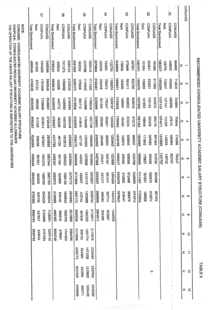
Table 6:Recommended Consolidated University Salary Structure (CONUASS)
Appendix 4
The computer programme is as follows: V(S)=POWER(S,-2r/σ2 )*(1/2r/σ2 )*POWER(K/((1+2r/σ2 ) ),(2r/σ2 +1) )
We used the first 4 columns, A, B, C, D, E (to represent) as follows:
A=S = salary (horizontal axis)
B=V(S) = financial values of retirement benefit (vertical axis)
C=K-S
D1= 2r/σ2
D2=K
Substituting these parameters into the above programme, we have
POWER(Ai,-D1) *(1/D1) *POWER(D2/(1+D1),(D1+1))
where i = 1,2,3,…,25 for University Senior lectureres .