Production System for Delayed Deterioration Inventories with Two-Level Production Rate, Stock-Dependent Demand Rate and Linear Holding Cost Under Trade Credit Policy
- M. L. Malumfashi
- A.M. Asma
- I. L. Kane
- B. Babangida
- T. A. Yusuf
- 81-104
- Feb 4, 2024
- Mathematics
Production System for Delayed Deterioration Inventories with Two-Level Production Rate, Stock-Dependent Demand Rate and Linear Holding Cost Under Trade Credit Policy
M. L. Malumfashi, A.M. Asma, I. L. Kane, B. Babangida, T. A. Yusuf
Department of Mathematics and Statistics, Umaru Musa Yar’adua University, PMB 2025, Katsina-Nigeria
DOI: https://doi.org/10.51584/IJRIAS.2024.90108
Received: 16 December 2023; Revised: 01 January 2024; Accepted: 04 January 2024; Published: 04 February 2024
ABSTRACT
This paper introduces an optimized total variable cost model for a production inventory system dealing with delayed deteriorating items. The model incorporates a two-level production rate and a stock-dependent demand rate, all operating under a trade credit policy. The demand rate remains constant during the inventory build-up period, but post-production, before deterioration, it varies based on product availability and nature. The inventory depletes to zero in the model’s final stage due to the combined impact of constant demand and deterioration rates. To characterize the optimality of the analytical results, the paper utilizes theorems and lemmas. The model’s dynamics are described by differential equations, which are solved using MATLAB. A numerical experiment is conducted to demonstrate the practicality of the developed models. Additionally, a sensitivity analysis is performed to illustrate how changes in selected system parameters affect the total variable costs determined in the numerical example. The paper concludes with suggestions and recommendations aimed at reducing the total variable cost. Ultimately, it is demonstrated that the developed model surpasses the one presented in the working paper. The proposed model could be used in inventory management and control of items that exhibit delayed in deterioration to minimises the total variable cost when sudden distraction of production process occurred as revealed by the the result presented.
Keywords: Delayed Deterioration, Two-level Production rate, Stock Demand, Linear Holding Cost, Trade Credit
INTRODUCTION
Production management constitutes a complex and critical aspect of business operations, especially in the context of developing countries. The intricacies of production are compounded by frequent disruptions resulting from conflicts, epidemics, terrorist acts, and other unforeseen events. These disruptions not only pose immediate threats to production processes but also necessitate a comprehensive approach to inventory control. The emergence of sudden and unpredictable events, exemplified by the impact of the COVID-19 pandemic on production environments, has heightened concerns within the field of production inventory control. In response to the imperative for effective models to navigate these challenges, researchers, as demonstrated by the work of Malumfashi et al. (2021a), have proposed an economic production quantity (EPQ) model specifically tailored for delayed deteriorating inventories. This model is designed to address the distinctive production problems arising from unforeseen events, such as the rapid onset of a pandemic. The focus on delayed deteriorating inventories underscores the temporal aspect of product deterioration, providing a more realistic representation of the challenges faced in managing inventory during prolonged disruptions. This research contributes to the development of strategies and models that are adaptive and resilient in the face of unpredictable events, offering valuable insights for enhanced production management practices.
Researchers, as outlined in Malumfashi et al. (2021b), have taken steps to refine the applicability of EPQ models by extending their efforts to incorporate variable production and demand rates. This adjustment offers a more realistic portrayal of global market dynamics, particularly when confronted with movement control orders enforced across affected countries. The model’s capacity to account for these nuanced scenarios enhances its effectiveness in addressing the intricacies of real-world production disruptions. Variable production rate denotes that the rate at which goods or services are produced can fluctuate over time. Such variability may stem from changes in demand, available resources, or other external factors. A production system featuring a variable production rate can adapt to diverse levels of demand or operational conditions, providing flexibility and responsiveness.
Linear holding cost pertains to a holding cost framework wherein the cost either rises or falls in direct proportion to the quantity of inventory held. In the realm of inventory management, holding costs encapsulate the expenditures linked to storing and keeping a specific quantity of goods. The concept of linear holding costs denotes a steady and linear correlation between the quantity of inventory and the corresponding holding costs. In the contemporary global business landscape, marked by numerous challenges and disruptions, the adoption of internationally recognized marketing policies, such as trade credit, becomes imperative. The integration of such policies into established models facilitates the determination of optimal total variable costs during production disruptions. This comprehensive approach not only accounts for the intricacies of the production process but also acknowledges broader economic and market dynamics that influence the optimal functioning of production management systems in the face of unforeseen events. Recent models, exemplified by the work of Yung (2007), have incorporated trade credit policies to address the complexities of production and demand dynamics. Yung (2007) investigated optimal retailer replenishment decisions under two levels of trade credit policy within the EPQ framework. Other notable contributions include Nita and Chetansinh’s (2018) EPQ model for deteriorating items with price-dependent demand and two-level trade credit financing, Majumder et al.’s (2019) EPQ model of substitute items under a trade credit policy, and Anindya et al.’s (2020) unreliable production-inventory model with varying demand under two-level trade credit policies. Majumder et al. (2020) extended this line of inquiry by developing an EPQ model of substitutable products under a trade credit policy with stock-dependent and random substitution. Ali et al. (2021) introduced an EPQ model for deteriorating items with a partial trade credit policy, considering price-dependent demand under inflation and reliability. Sunit et al. (2021) explored an EPQ model with two-level trade credit and multivariate demand, incorporating the effects of system improvement and preservation technology. Kumar et al. (2021) developed an EPQ model with a learning effect for imperfect quality items under trade-credit financing. A notable observation is that many existing models focused on instantaneous items, which may be less realistic in today’s market. In contrast, the concept of delayed deterioration has been acknowledged as a more accurate representation of contemporary product quality maintenance. Delayed deterioration refers to a scenario where the degradation of a product occurs over time, but the impact is not immediate, introducing a time lag between the initiation of the deterioration process and its full realization. This concept is particularly relevant in inventory management and production systems, reflecting the gradual degradation of items over time rather than an instantaneous decline in quality.
Stock-dependent demand rate refers to the phenomenon where the demand for a product is influenced by the current stock level. Essentially, fluctuations in the stock of a particular item can lead to changes in the demand for that item. This concept holds significant importance in inventory management, where alterations in stock levels can directly affect the consumption or sale rate of items. Shah et al. (2016) addressed this concept by developing an inventory model within an imperfect production system, taking into account demand sensitivity to both price and stock levels. Defective items produced underwent rejection, reworking, or refunding if already delivered to customers. Ruchi and Buttar (2021) extended the classical EPQ model by considering the impact of an epidemic on a production unit subjected to stochastic lockdown times. The expected production time was evaluated using a continuous probability density function. The study aimed to determine the optimal arrangement for the production system, minimizing the expected total cost per unit of time under specific conditions. The model treated epidemic-related lockdown times as stochastic, acknowledging that machine breakdowns affect both the manufacturer and customers, whereas disasters like epidemics affect both production and demand. During regular production uptime, demand depends on stock levels and decreases with selling prices, but during disasters like epidemics, selling prices become irrelevant, and demand depends solely on stock levels. Hesham and Ahmed (2022) introduced a generalized production-inventory model that allows for variable production, demand, and cost rates by relaxing the assumption of constant values for all input parameters. The model considered demand rates, production rates, and all cost rates as either dependent or decision variables. Demand was assumed a linear function of both the selling price and the average stock level. Setup costs per production run and production costs per unit were considered nonlinear functions of the production rate. Holding costs were assumed linear functions of the production cost and the duration of storage time. Nita et al. (2022) developed an EPQ model incorporating price-sensitive stock-dependent demand and carbon emissions, considering investments in green and preservation technologies. The model was studied under three scenarios: (i) with green technology investment, (ii) with preservation technology investment, and (iii) with both green and preservation technology investments.
The literature review indicates the existence of numerous economic production quality models developed under varied assumptions, encompassing variable production rates, stock-dependent demand rates, linearly increasing functions of time for holding costs, and trade credit policies. Notably, Malumfashi et al. (2022) take care of the variable production, exponential demand rate and linear holding cost, while Malumfashi and Ali. (2023) addressed both variable production and stock-dependent demand, incorporating several realistic assumptions such as stock dependent demand rate, two-phase production and demand rates. However, their works did not account for linear holding costs and the prevalent trade policy known as trade credit. This study fills this gap by introducing a production inventory model tailored for delayed deteriorating items. The model features a two-level production rate, stock-dependent demand rate, and a linearly increasing function of time for holding costs, all operating under a trade credit policy. The aim is to provide a solution for the production challenges arising during a disrupted production period.
Notations
A The set-up cost per production run.
α The production rate in unit per unit time.
μ The demand rate during inventory build-up in unit per unit time.
μ1 The demand rate after production before deterioration starts in unit per unit time.
μ2 The demand rate at the point deterioration starts in unit per unit time.
a Production rate changing parameter.
i Inventory carrying charge.
θ Deterioration rate
C Unit cost per item
Cθ The cost of deterioration
H The total holding cost.
Ie The interest earned by the wholesaler.
IC The interest charged by the producer.
Y1 The inventory level at the point instantaneous change of production rate occurs.
Y2 The inventory level at the end of the production period.
Y3 The inventory level at the point deterioration starts.
Y(t) The inventory level during inventory build-up before production rate changes, where 0 ≤t ≤ T1.
Y1(t) The inventory level after production rate changes, where T1 ≤t ≤ T2.
Y2(t) The inventory level after production stops before deterioration starts, where T2 ≤t ≤ T3.
Y3(t) The inventory level within deterioration period, where T3 ≤t ≤ T.
Ti Unit time in periods (i ∈ {1,2,3}).
T Total cycle length (decision variable).
Z Total variable cost (decision variable).
EPQ Economic production quantity per cycle (decision variable).
2.2 Assumptions
- Production starts instantaneously.
- Production rate changes instantaneously.
- Unconstrained Capital Supplies.
- Shortage not
- Discarded all Defective Items after inspection.
- The Demand Rate within the Production Period is less than the production rate.
- The Production Rate is of two phases with a Two-level production rate defined as a function.
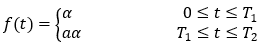 for a∈{(0,1)∪(1,2)}
- The demand rates μ and μ2 (within production and deterioration periods respectively).
- The demand rate μ1 (after inventory build-up period before deterioration set in) is stock-dependent and defined as μ1=ρ+βY2 (t), where ρ is a constant demand rate and β is the stock dependent parameter, β∈[0,1].
- The holding cost for an item is linearly increasing function of time defined as Ch=c1+c2t, where c1 is a constant holding cost and c2 is a holding cost that change linearly to time.
- Time horizon is finite.
- T-T1<1 (It is unreasonable to have continues deterioration up to one year)
- Ic≥Ie,
- If T≤M, the account is settled at T= M , the wholesaler pays off all units sold and keep his/her profits and starts paying for the interest charges on the items in stock with Ic. When T≤M, the account is settled at T= M and the wholesaler does not need to pay any interest charge.
MODELLING
Figure 1 shows how the inventory level varies with time due to both change in production, demand, and deterioration rates. The production starts at time at t=0 and changes at t=T1. The production and demand rates during the time interval [0, T1] are α and μ respectively and the inventory rich a level Y1 at time T1. During the interval [T1,T2 ], the inventories continue accumulating at a rate aα – μ due to change in production rate (increase or decrease with the parameter a) while demand remain the same as initial. The demand within the interval [T2,T3] is stock dependent(μ1=ρ+βY2 (t)). Deterioration starts when the inventory drop to Y3 at time T3. The inventories drop to zero due to both demand and deterioration time T.
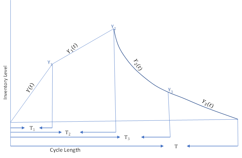
Figure 1: Graphical representation of the inventory system
The equations that describe the situations of the four periods of the model above are as follows.
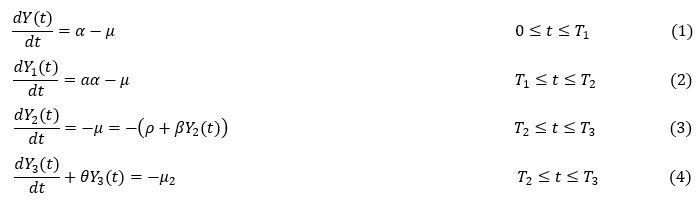
The solutions of the ordinary differential equation (ODE) given in Eq. (1) which described the situation within the time period 0≤t≤T1 is obtained using the boundary conditions Y(0)=0 and Y(T1)=Y1 as
Y(t)=(α-μ)t (5)
The solution of the ODE given in Eq. (2) which described the situation within the time period T1≤t≤T2 is obtained using the boundary conditions Y1 (T1)=Y1 and Y1 (T2)=Y2 as
Y1 (t)=(aα-μ)(t-T1 )+(α-μ) T1 (6)
Eq. (3) is solved considering the boundary conditions Y2 (T2)=Y2 and Y2 (T3)=Y3 and obtained as
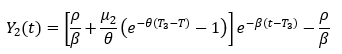 (7)
(7)
Where the total number of items at the point deterioration sets in Y3 is calculated as
![]()
And the solution of the ODE which described the situation of the deterioration period T3≤t≤T is under the boundary conditions Y2 (T3)=Y3 and Y2 (T)=0 is obtained using the method of integrating factor as
![]() (8)
(8)
The cost of deterioration, which is a multiple of a cost per unit item and difference between the number of items remain at the very time deterioration sets in and the number of items demanded within the period of deterioration is determined as
![]() (9)
(9)
Holding Cost, this is the cost associated with the inventory carrying charge and the cost of holding items from the first item produced to the last item to be sold which is a multiple of inventory carrying charge per unit item, cost of hold per unit item (this is a linear function of time) and the total number of items stored determined as
 (10)
(10)
Substituting Eq.s (5-8) in Eq.s (10) and simplify,
Case1: T2≤M≤T3
When the credit period is within the period after production before deterioration sets in, this prevailed that the wholesaler needs to settle his account before deterioration sets in.
The commission paid to the wholesaler when he settled the account before the end of the credit period is calculated as
![]() (12)
(12)
The interest earned by manufacturer is the amount charged from the wholesaler for the remaining items at the time deterioration sets in which is calculated as
 (13)
(13)
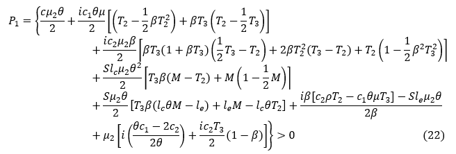
The Total Variable Cost Per cycle Length is a sum set up cost per cycle length, deterioration cost per cycle length, holding cost per cycle length and commission paid per cycle length minus interest earned per cycle length.
![]() (14)
(14)
Substituting Eq. (9), (11), (12) and (13) in Eq. (14)
Case 2: T3≤M≤T
When the credit period begins immediately after production period and ends at the end of the cycle length (at the time the store of the manufacturer depleted to empty).
The commission payable to the wholesaler when he settled the account at least at the end of the cycle length T is obtained below
![]()
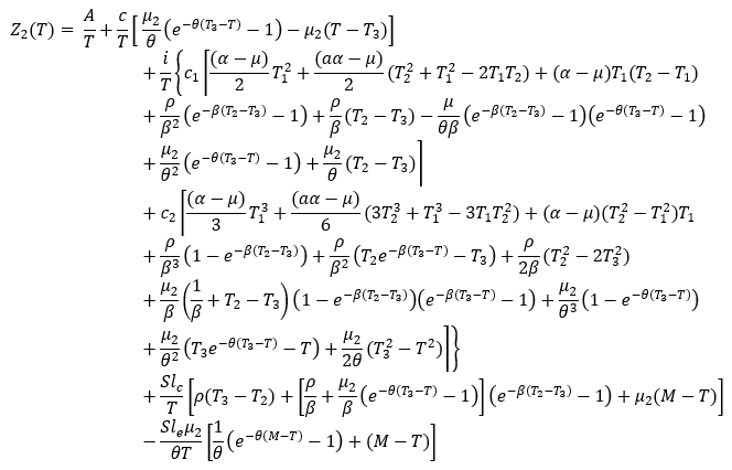
The interest earn by manufacturer is the amount charged from the wholesaler for the remaining items at the time manufacture sold all the on-hand inventory which is calculated as

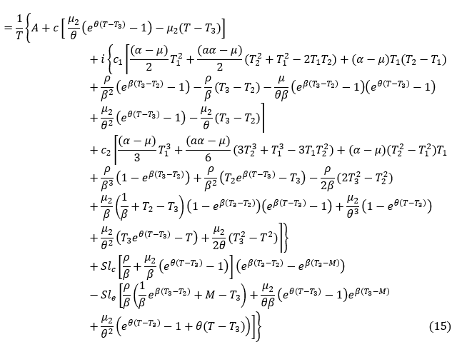
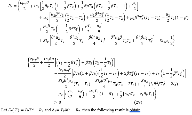
The total Variable Cost in this case is calculated as Eq. (16) below
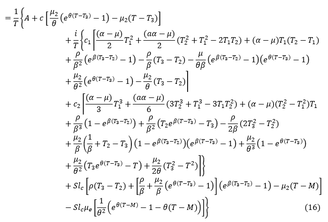
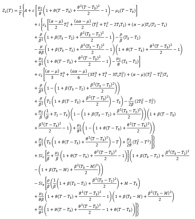
Utilizing quadratic approximation for the exponential terms in Eq. (15) and (16) to obtain
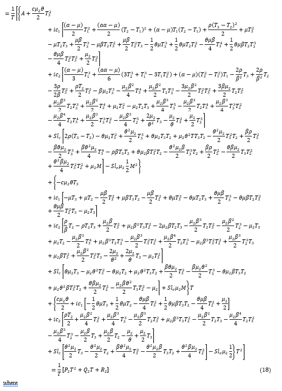
OPTIMALITY CONDITION
Case 1: (T2≤M≤T3)
The necessary and sufficient conditions that minimize Z1 (T) are respectively, ![]() =0 and
=0 and ![]()
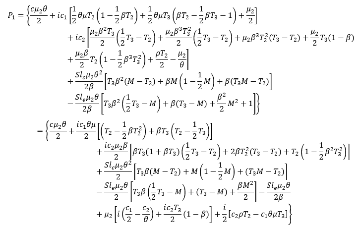
The first derivatives of the total variable cost, in Eq. (17), with respect tois as follows.
 (19)
(19)
Therefore, ![]() =0 gives the following nonlinear equation in terms T
=0 gives the following nonlinear equation in terms T
![]() (20)
(20)
which implies
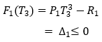
P1 T2-R1=0 (21)
Theorem 1.
![]()
Proof:
Since βM2→0, then
Let F1 ( T)=P1 T2-R1 and ∆1=P1 T33-R1, then the following result is obtain
Theorem 2. For T2≤M≤T3,
(i) If ∆1≤0, then the solution of T∈[T3, ∞) (say T*1) which satisfies (21) not only exists but also is unique.
(ii) If ∆1>0, then the solution of T∈[T3, ∞) which satisfies (21) does not exist.
Proof of (i). From Eq. (21), we define a new function F1 (T) as follows
![]() (23)
(23)
Taking the first-order derivative of F1 (T) with respect to T∈[T3, ∞), we have
![]()
We obtain that F1 (T) is an increasing function of in the interval T∈[T3, ∞), Moreover, we have
![]()
and
Now F1 ( T3 )≤0. Therefore, by applying intermediate value theorem, there exists a unique T*1∈[T3,∞) such that F1 (T*1)=0 . Hence T*1 is the unique solution of (21). Thus, the value of T (denoted by T*1) can be found from (21) and is given by
 (24)
(24)
Proof of (ii). If ∆1>0, then from (21), we have F1 ( T)>0. Since F1 ( T) is an increasing function of T∈[T3,∞) then F1 ( T)>0 for all T∈[T3,∞) Thus, we cannot find a value T∈[T3,∞) of such that F1 (T)=0. This completes the proof.
Theorem 3. When T2≤M≤T3
(i) If ∆1≤0, then the total variable cost Z1 (T) is convex and reaches its global minimum at the point T*1∈[T3,∞), where T*1 is the point which satisfies (21).
(ii) If ∆1>0, then the total variable cost Z1(T) has a minimum value at the point T*1=T
Proof of (i). When ∆1≤0, we see that T*1 is the unique solution of (21) from Theorem 2(i). Taking the second derivative of Z1(T) with respect to and then finding the value of the function at the point T*1, we obtain
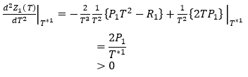 (25)
(25)
We thus conclude from (25) and Theory 2 that Z1(T*1) is convex and T*1 is the global minimum point of Z1(T). Hence the value of T in (24) is optimal.
Proof of (ii). When ∆1>0, then we know that F1 (T)>0 for all T∈ [T3,∞). Thus, ![]() for all ∈ [T3,∞) which implies Z1(T) is an increasing function of T. Thus Z1(T) has a minimum value when T is minimum. Therefore, Z1(T) has a minimum value at the point T=T3. This completes the proof.
for all ∈ [T3,∞) which implies Z1(T) is an increasing function of T. Thus Z1(T) has a minimum value when T is minimum. Therefore, Z1(T) has a minimum value at the point T=T3. This completes the proof.
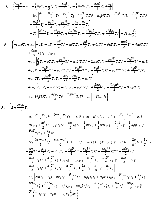
Case 2: (T3≤M≤T)
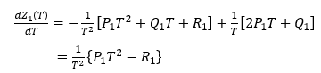
The necessary and sufficient conditions that minimize Z2(T) are respectively, (dZ2 (T))/dT=0 and (d2Z2(T))/(dT2)>0
The first derivatives of the total variable cost, in (18), with respect tois as follows.
 (26)
(26)
Therefore, (dZ2 (T))/dT=0 gives the following nonlinear equation in terms T
![]() (27)
(27)
which implies
P2 T2-R2=0 (28)
Theorem 4.
![]()
Proof:
Theorem 5. For T3≤M≤T,
(i) If ∆2≤0, then the solution of T∈ [M,∞) (say T*2) which satisfies (28) not only exists but also is unique.
(ii) If ∆2≤0, then the solution of T∈ [M,∞) which satisfies (28) does not exist.
Proof of (i). From (28), we define a new function F2(T) as follows
F2(T)=P2 T2-R2, T∈ [M,∞) (30)
Taking thet first-order derivative of F2(T) with respect to T∈ [M,∞), we have
![]()
We obtain that F2(T) is an increasing function of T in the interval [M,∞) Moreover, we have
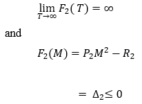
Now F2 (M2)≤0. Therefore, by applying intermediate value theorem, there exists a unique T*2∈ M2,∞) such that F2 (T*2)= 0. Hence T*2 is the unique solution of (28). Thus, the value of T (denoted by T*2) can be found from (28) and is given by
![]() (31)
(31)
Proof of (ii). If ∆2>0, then from (28), we have F2( T)>0 . Since F2( T) is an increasing function of T∈ [M,∞) then F2(T)>0 for all T∈ [M,∞) Thus, we cannot find a value of T∈ [M,∞) such that F2( T)=0. This completes the proof.
Theorem 6. When T3≤M≤T
(i) If ∆2≤0, then the total variable cost Z2(T) is convex and reaches its global minimum at the point T*2∈ M2,∞), where T*2 is the point which satisfies (28).
(ii) If ∆2>0, then the total variable cost Z2(T) has a minimum value at the point T*2=M2.
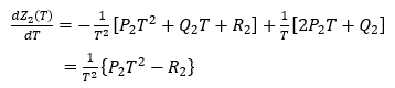
Proof of (i). When ∆2≤0, we see that T*2 is the unique solution of (2) from Theorem 5(i). Taking the second derivative of Z2(T) with respect to and then finding the value of the function at the point T*2, we obtain
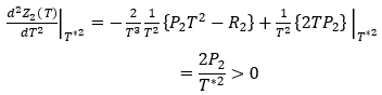 (32)
(32)
We thus conclude from (32) and Theory 2 that Z2(T*2) is convex and T*2 is the global minimum point of Z2(T). Hence, the value of T in (31) is optimal.
Proof of (ii). When ∆2>0, then we know that F2( T)>0 for all T∈ [T3,∞) . Thus, ![]() for all T∈ [T3,∞) , which implies F2( T) is an increasing function of T. Thus F2( T) has a minimum value when T is minimum. Therefore, F2( T) has a minimum value at the point T=T3. This completes the proof.
for all T∈ [T3,∞) , which implies F2( T) is an increasing function of T. Thus F2( T) has a minimum value when T is minimum. Therefore, F2( T) has a minimum value at the point T=T3. This completes the proof.
NUMERICAL EXPERIMENTS
These proposed models are illustrated by performing the numerical experiments as follows.
The parameter values are adopted from Malumfashi and Ali. (2023) and add the values of parameters absent in their work (lc, le, and ) as presented in the Table 1.
Table 1 Experiment parameters
| Parameter | Value | Parameter. | Value |
| Α | N3,300 per production run | T1 | 0.547945 years |
| I | 1.2 | T2 | 0.82192 years |
| Μ | 3,500 units per unit time | T3 | 0.90411 years |
| μ 2 | 2,100 units per unit time | A | 0.1 |
| ρ | 2,500 units per unit time | C | 140 per unit |
| θ | 0.2 units per unit time | lc | N30 per unit |
| le | N20 per unit | β | 0.3 |
| α | 6000 units per production run |
RESULTS
The problem described by the parameters above is solve upon substituting the parameters values in Eq.s (15), (16), (24) and (31) respectively. The optimal solutions of the best cycle lengths and the optimal total variable cost per production runs are obtained and shown in Table 2.
Table 2. Optimal solution
| Variable | Value |
| Z1 | N67,117.5422 per cycle |
| T*1 | 1.0066 years |
| Z2 | N59,929.8902 per cycle |
| T*2 | 0.9919 years |
Comparison between the proposed model, Malumfashi et al. (2021a) and Malumfashi and Ali. (2023)
The aim of both this proposed models, Malumfashi et al. (2021a) and Malumfashi and Ali. (2023) is to minimises the total variable cost within the distracted cycle length. The total variable cost = N59,929.8902 obtained here is minimum to that obtained in the Malumfashi et al. (2021a) and Malumfashi and Ali. (2023) and that of obtained in the first model of this work. Similarly, the cycle length = 0.9919 obtained in the second model here is minimum. As such, this model improves upon that developed in in the literature and the additional assumptions proved to be more realistic. This shows that, the total variable cost will be at its minimum level if the trade credit period reaches deterioration period. As such, the result roved that this proposed mode is optimal to all the existing models for delayed deteriorating items solving the sudden distraction of the production process and revealed that producers would operated at lowest cost if the trade credit period is allowed to runs up to the deterioration period.
SENSITIVITY ANALYSIS
Using the results obtained in the above experiment, the sensitivity analysis is performed to study the effect of changes in some system’s parameters on the obtained optimal solutions and the results are shown below.
Table 3 shows the effect of change in set-up cost A on the total variable cost when the wholesaler settled the account before deterioration set in and the total variable cost when the wholesaler settled the account within the deterioration period . Both the total variable costs per cycle length and increase as the set-up cost (A) increases and decreases in the reverse case. In a normal circumstance, any change in set-up cost impacts the total variable cost. This indicates that manufacturers should make sure that the production rate is at maximum when the set-up cost is high.
Table 3: effect of change in set-up cost A on the total variable cost Z1 and Z2
| % change in A | % change in Z1 | % change in Z2 |
| +50 | 34.9674 | 5.1159 |
| +25 | 17.9824 | 2.4168 |
| 0 | 0.0000 | 0.0000 |
| −25 | −18.2922 | −3.8679 |
| 50 | 39.2709 | 4.2348 |
Table 4 shows the effect of change in cost per unit item C on the total variable cost Z1 and Z2. As the cost per unit item (C) increases, the total variable costs per cycle length Z1 and Z2. In a real-life situation, any increase in the cost of an item will increase the total variable cost per cycle. As such, it is recommended that manufacturers ensure that the EPQ is at its maximum to lower the cost ratio which will eventually reduce the total variable cost.
Table 4: Effect of change in cost per unit item C on the total variable cost Z1 and Z2
| % change in C | % change in Z1 | % change in Z2 |
| +50 | 13.6362 | 10.2407 |
| +25 | 7.1978 | 3.4155 |
| 0 | 0.0000 | 0.0000 |
| −25 | −9.8568 | −3.3228 |
| 50 | 18.7672 | −5.2967 |
Table 5 shows the effect of change in production rate μ on the total variable cost Z1 and Z2. As the production rate (α) increases, both the total variable costs per cycle Z1 and Z2 increase. This means that any adjustment in production rate has a similar impact on both total variable costs per cycle length in both models. This reveals the need to of extra care on the production rate at any stage.
Table 5: effect of change in production rate μ on the total variable cost Z1 and Z2
| % change in α | % change in Z1 | % change in Z2 |
| +50 | 0.3497 | 9.5273 |
| +25 | 0.0965 | 4.7506 |
| 0 | 0.0000 | 0.0000 |
| −25 | −0.1351 | −4.7238 |
| 50 | −0.2721 | −9.4205 |
Table 6 shows the effect of change in inventory carrying charge i on the total variable costs Z1 and Z2. As the inventory carrying charge (i) increases, the total variable cost per cycle of the first model Z1 increases and that of the second Z2 also increases. It is clear in real-life situations that any increase in carrying charge increases the total variable cost. It is recommended that manufacturers make sure the minimum inventory carrying charge to optimise the total variable cost.
Table 6: effect of change in inventory carrying charge on the total variable costs Z1 and Z2.
| % change in i | % change in Z1 | % change in Z2 |
| +50 | 0.0271 | 14.2646 |
| +25 | 0.01700 | 7.1386 |
| 0 | 0.0000 | 0.0000 |
| −25 | −0.0324 | −7.1465 |
| 50 | −0.0865 | −14.2974 |
Table 7 shows the effect of the change in deterioration rate θ on the total variable costs Z1 and Z2. As the deterioration rate (θ) increases, both the total variable costs per cycle length Z1 and Z2 increases. Naturally, any increase in the deterioration rate increases the total variable cost, also any change in the deterioration rate has a significant impact on the quantity produced in a cycle length. The manufacturer should provide adequate raw materials and excellent storage facilities so that the rate of deterioration is low.
Table 7: effect of the change in deterioration rate θ on the total variable costs Z1 and Z2.
| % change in θ | % change in Z1 | % change in Z2 |
| +50 | −0.0271 | −14.2646 |
| +25 | −0.01700 | −7.1386 |
| 0 | 0.0000 | 0.0000 |
| −25 | 0.0324 | 7.1465 |
| 50 | 0.0865 | 14.2974 |
CONCLUSION
The findings of this research highlight the feasibility of aligning the trade credit period with the deterioration period to effectively minimize the total variable cost within the economic production quantity model for delayed deteriorating items with stock-dependent demand rate and linear holding cost. This strategic alignment emerges as a practical approach for optimizing cost-effectiveness in the face of prolonged deterioration periods. Furthermore, the study underscores the reliability of integrating trade credit policies, especially when coupled with stock-dependent demand rates and linear holding costs, within the economic production quantity model for delayed deteriorating items. This integration proves beneficial in enhancing the overall efficiency of the production and inventory management system. Based on the results, the research suggests the potential for further refinement by developing similar models with a range of optional trade credit periods. Such an exploration could unveil the most optimal trade credit period corresponding to the minimization of the total variable cost. This recommendation opens avenues for future research to delve deeper into the nuances of trade credit policies and their impact on economic production quantity models under various conditions, providing valuable insights for practitioners and decision-makers in the field of production management.
REFERENCES
- Ali, A. S. Leopoldo, E. C. Kumar, M. and Cespedes, M. (2021). An economic production quantity (EPQ) model for a deteriorating item with partial trade credit policy for price dependent demand under inflation and reliability. Yugoslav Journal of Operations Research, 31(2), 139–151. DOI: https://doi.org/10.2298/YJOR200515036S.
- Anindya, M., Brojeswar, P. and Kripasindhu, C. (2020). Unreliable EPQ model with variable demand under two-tier credit financing. Journal of Industrial and Production Engineering, 37(7), 370–386. https://doi.org/10.1080/21681015.2020.1815877.
- Hesham, K. A. and Ahmed, M. G. (2022). A Generalized Production-Inventory Model with Variable Production, Demand, and Cost Rates. Arabian Journal for Science and Engineering, 47, 3963–3978. https://doi.org/10.1007/s13369-021-06516-4.
- Kumar, M. J. Mandeep, M., Isha, S. and Rita, Y. (2021). EPQ model with learning effect for imperfect quality items under trade-credit financing. Yugoslav Journal of Operations Research, 31(2), 235–247. DOI: https://doi.org/10.2298/YJOR2002016010Y.
- Majumder, P., Bera, U. K. and Maiti, M. (2020). An EPQ model of substitutable products under trade credit policy with stock dependent and random substitution. OPSEARCH, 57, 1205-1243. https://doi.org/10.1007/s12597-020-00449-6.
- Majumder, P., Bera, U. K. and Manoranjan, M. (2019). An EPQ model of deteriorating substitute items under trade credit policy. International. Journal of Operation Research, 34(2), 161–212. https://doi.org/10.1504/IJOR.2019. 097576.
- Malumfashi, M.L. and Ali, M.K.M. (2023) ‘A production inventory model for non-instantaneous deteriorating items with two-phase production period, stock-dependent demand and shortages’, Int. J. Mathematics in Operational Research, Vol. 24, No. 2, pp.173–193.
- Malumfashi, M. L., Ismail, M. T., & Ali, M. K. M. (2022). An EPQ Model for Delayed Deteriorating Items with Two-Phase Production Period, Exponential Demand Rate and Linear Holding Cost. Bulletin of the Malaysian Mathematical Sciences Society, 45(Suppl 1), 395-424.
- Malumfashi, M. L., Ismail, M. T., Rahman, A., Sani, D., & Ali, M. K. M. (2021a). An EPQ model for delayed deteriorating items with variable production rate, two-phase demand rates and shortages. In Modelling, Simulation and Applications of Complex Systems: CoSMoS 2019, Penang, Malaysia, April 8–11, 2019 (pp. 381–403). Springer Singapore.
- Malumfashi, M.L., Ismail, M.T., Bature, B., Sani, D., Ali, M.K.M. (2021b). An EPQ Model for Delayed Deteriorating Items with Two-Phase Production Period, Variable Demand Rate and Linear Holding Cost. In Modelling, Simulation and Applications of Complex Systems. CoSMoS 2019. Penang, Malaysia, April 8–11, 2019 (pp. 404–432). Springer Singapore.
- Nita, H. S. and Chetansinh, R. V. (2018). An EPQ model for deteriorating items with price dependent demand and two-level trade credit financing. Revista Investigación Operacional, 39(2), 170-180.
- Nita S., Ekta, P. and Kavita, R. (2022). EPQ model to price-sensitive stock dependent demand with carbon emission under green and preservation technology investment. Economic Computation and Economic Cybernetics Studies and Research, 56(1), 209-222.
- Ruchi, S. and Buttar, G. S. (2021). An EPQ Model of Stock Dependent Demand Subject to Epidemic with Stochastic Lockdown Time. Turkish Journal of Computer and Mathematics Education, 12(2), 2859-2867.
- Shah, N.H., Patel, D. G. and Shah, D. B. (2016). EPQ model for returned/reworked inventories during imperfect production process under price-sensitive stock-dependent demand. International Journal of Operation Research, 18, 343-359. https:// doi.org/10.1007/s12351-016-0267-4.
- Sunit K., Sushil, K. and Rachna, K. (2021). An EPQ model with two-level trade credit and multivariate demand incorporating the effect of system improvement and preservation technology. Malaya Journal of Matematik, 9(1), 438-448. https://doi.org/10.26637/MJM0901/0074.
- Yung, F. H. (2007). Optimal retailer’s replenishment decisions in the EPQ model under two levels of trade credit policy. European Journal of Operational Research, 176, 1577–1591.