
Enhancing Magnetohydrodynamic Stability in Channel Flows through Porous Media Incorporating Darcy-Forchheimer Modifications into the Orr-Sommerfeld Analysis
- Akindele M. Okedoye
- Akpabokigho L. Panya
- Muhammad M. Lawal
- 135-151
- Jun 5, 2024
- Mathematics
Enhancing Magnetohydrodynamic Stability in Channel Flows through Porous Media Incorporating Darcy-Forchheimer Modifications into the Orr-Sommerfeld Analysis
Akindele M. Okedoye1, Akpabokigho L. Panya2 and Muhammad M. Lawal1
1Department of Mathematics, Federal University of Petroleum Resources, Effurun, Delta State, Nigeria
2Department of Mathematics, Delta State University of Science and Technology, Ozoro, Delta State, Nigeria
DOI: https://doi.org/10.51584/IJRIAS.2024.905012
Received: 08 April 2024; Revised: 27 April 2024; Accepted: 01 May 2024; Published: 04 June 2024
ABSTRACT
This research paper investigates the stability characteristics of magnetohydrodynamic (MHD) flow within channels filled with porous media. Specifically, the study explores modifications to the classical Orr-Sommerfeld equation using the Darcy-Forchheimer model to account for the presence of porous media. The analysis aims to elucidate the combined influence of porous media and magnetic fields on flow stability in such systems. Numerical simulations and analytical techniques are employed to assess the impact of varying parameters on the stability behavior of the flow. The study revealed that the velocity profile increases with increase in Schmidt and Prandtl’s number and stabilizes with the increase in Grashof number and the buoyancy. The temperature profile increases with Reynold’s Number and Hartmann number. It stabilizes with Schmidt, Prandtl and Grashof number. The profile of species concentration stabilizes with thermo-phoretic parameter, Prandtl number and Darcy-Forchheimer’s parameter augumentation.
Keywords— Darcy-Forchheimer model, Orr-Sommerfeld analysis, Magnetohydrodynamic, Viscous flow, Porous Media, Stability, Channel
INTRODUCTION
Magnetohydrodynamic (MHD) flow, characterized by the interaction between electrically conducting fluids and magnetic fields, finds widespread applications in engineering and scientific research. In many practical scenarios, such flows occur within channels filled with porous media, introducing additional complexities to the flow behavior. Understanding the stability of such flows is crucial for the design and operation of various engineering systems. This study focuses on investigating the stability of MHD flow in channels occupied by porous media, with a particular emphasis on incorporating the Darcy-Forchheimer model into the classical Orr-Sommerfeld analysis. Stability analysis of flow, pioneered by Reynolds, Orr, and Sommerfeld, remains integral to fluid mechanics (Reynolds [1]; Orr [2]; Sommerfeld [3]).
Magnetohydrodynamic (MHD) flow, involving electrically conducting fluids in magnetic fields, finds applications in various industries (Hayat et al. [4]). The flow through porous media is reported extensively by the following literature review by the studies, Umavathi and Veershetty [5], Krishnamurthy [6] and Haider et al. [7]. In the modeling of the two-dimensional magnetohydrodynamic boundary layer flow in a channel with porous walls, Okedoye [8] studied the analytical analysis of steady MHD free convective heat and mass transfer flow past a semi-infinite vertical porous plate in porous medium has been studied including the Dufour and Soret effects. Ibrahim [9] investigated the effects of mass transfer, radiation, Joule heating, and viscous dissipation on steady MHD Marangoni convection flow over a flat surface with suction and injection. MHD effects on heat transmission over a stretching sheet immersed in a porous medium with variable viscosity and viscous dissipation were studied by Hunegnaw and Naikoti [10]. Adesanya et al. [11] investigated the Thermodynamics Analysis of Hydromagnetic Third Grade Fluid Flow through a Channel Filled with Porous Medium. Again, Okedoye [12] investigated the analytical calculation of entropy generation due to unsteady magnetohydrodynamic heat and mass transfer in MHD flow past an infinite vertical oscillating plate was considered, taking account of the presence of free convection with mass transfer. In a micropolar fluid with radiation, Mabood et al. [13] investigated the effects of Soret effects and non-uniform heat sources/sinks on MHD non-Darcian convective flow past a stretched sheet. Darcy’s Law and its modification by Forchheimer are fundamental in understanding such flows Liu [14]. The Darcy–Forchheimer model addresses both viscous and inertial effects (Shehzad et al. [15]). Hayat et al. [16] analyzed Maxwell fluid through temperature dependent thermal conductivity and heat flux of Darcy–Forchheimer flow through Cattaneo-Christov theory while Gbadeyan and Opanuga [17] worked on inherent irreversibility analysis in a buoyancy induced MHD couple stress fluid. Their results confirmed that increase in buoyancy force and suction/injection increases fluid velocity and temperature. The effects of slip on the MHD flow of a dusty fluid across a stretching sheet through porous space were investigated by Abbas et al. [18]. The impact of nonlinear radiative heat and mass transfer on MHD flow across a stretching surface with changing conductivity and viscosity was investigated by Okedoye and Salawu [19]. The flow in porous media is a crucial aspect across various disciplines, including engineering, geosciences, and biology (Kumar & Varma [20]; Menni et al. [21]. Falana and Alao [22] examined the Similarity Solution of Heat and Mass Transfer Flow of a Nanofluid across a Porous Plate in a Darcy-Forchheimer Flow. Sharma and Mishra [23] studied the impact of MHD and internal heat generation/absorption on micropolar fluid moving along a stretchable sheet. Eid et al. [24] investigated homogeneous-heterogeneous in the MHD flow of a non-Newtonian Prandtl fluid via a permeable linear horizontal expandable (shrinkable) surface. Panya et al. [25] studied MHD Darcy-Forchheimer Slip Flow in a Porous Medium with Variable Thermo-Physical Properties. They find that when the porosity parameter is increased, the velocity of the fluid decrease, while temperature profile and skin friction decrease.
As reported in the above considerations, previous studies have extensively explored the stability of MHD flows and the influence of porous media separately. However, limited research has been conducted on the combined effects of both factors. Notably, Darcy-Forchheimer modifications to the classical equations governing flow in porous media have been proposed, providing a framework for analyzing flow stability in such systems. Additionally, the Orr-Sommerfeld equation has been widely used to study the stability of viscous flows, but its applicability to MHD flows within porous media remains underexplored. By incorporating the Darcy-Forchheimer formulation, the study aims to provide insights into the combined influence of porous media and magnetic fields on flow stability in such systems.
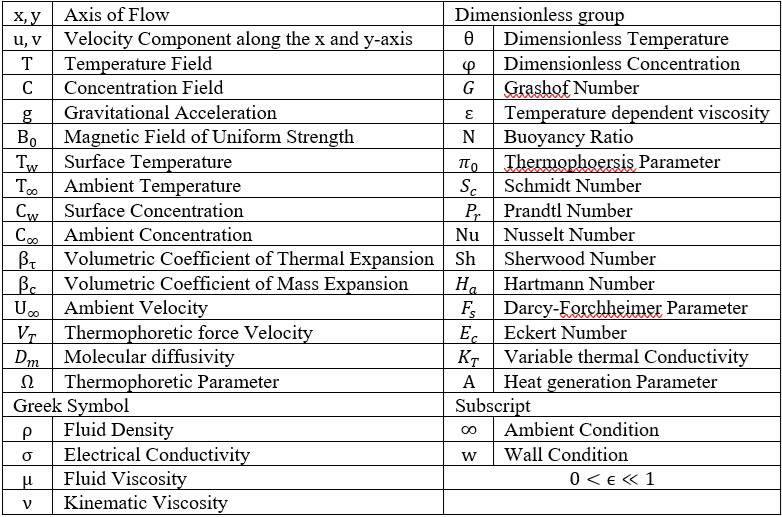
NOMENCLATURE
PROBLEM FORMULATION
Consider an unsteady MHD laminar fluid regime of viscous incompressible fluid with heat and mass transfer over a porous medium. A uniform magnetic field of intensity B is imposed perpendicular to the flow direction and x “and ” y-axis are parallel and normal to the surface of plate respectively. The induced magnetic field is assumed to be small compared to the applied magnetic field. Let u “and ” v be the fluid velocity tangentially and normally respectively. The ambient temperature of the fluid and the concentration far from the surface are taken as T∞ “and ” C∞ respectively. While the surface below the fluid is heated by convection from the fluid having initial temperature Tw with concentration Cw. It is assumed that the porous medium is homogeneous and isotropic and saturated. A sketch of the physical model and the flow schematics are given in Figure 1. In Abdul Hakeem et al (2014) non-uniform heat source/sink (q”’) and thermo-phoretic velocity (VT) are given by
\( q”’ = \kappa u w_{xx} \nu A^* (T_w – T_\infty) b x u – U + B (T – T_\infty) V T = k’ \nu \tau \frac{\partial T}{\partial y} \) (1)
Following Arunachalam and Rajappa (1978) and Chaim (1998) the thermal conductivity \( K_T = k_T T_\infty \) (2)
Using the boundary-layer approximations the continuity, momentum, energy, and mass species equations governing the type of flow under consideration become:
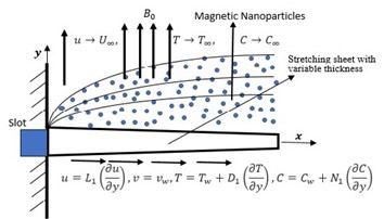
Figure 1: Flow Geometry of problem
\[ \frac{\partial u}{\partial t} + u \frac{\partial u}{\partial x} + v \frac{\partial u}{\partial y} = -\frac{1}{\rho} \frac{\partial p}{\partial x} + \nu \frac{\partial^2 u}{\partial x^2} + \frac{\partial^2 u}{\partial y^2} – \frac{\sigma \mu B^2 x}{\rho k} u – U \mp g \frac{\rho \nu K_1}{u} u – U + g \rho \beta \tau (T – T_\infty) + \beta_c (C – C_\infty) \] (3)
\[ \frac{\partial v}{\partial t} + u \frac{\partial v}{\partial x} + v \frac{\partial v}{\partial y} = -\frac{1}{\rho} \frac{\partial p}{\partial y} + \nu \frac{\partial^2 v}{\partial x^2} + \frac{\partial^2 v}{\partial y^2} – \frac{\sigma \mu B^2 x}{\rho k} v – U \mp g \frac{\rho \nu K_1}{u} v – U \] (4)
\[ \rho c_p \frac{\partial T}{\partial t} + u \frac{\partial T}{\partial x} + v \frac{\partial T}{\partial y} = \frac{\partial}{\partial y} \left( k_T T_\infty \frac{\partial T}{\partial y} \right) + \mu \left( \frac{\partial u}{\partial y} \right)^2 + k \left( u w_{xx} \nu A^* (T_w – T_\infty) b x u – U + B (T – T_\infty) \right) \] (5)
\[ \frac{\partial C}{\partial t} + u \frac{\partial C}{\partial x} + v \frac{\partial C}{\partial y} = D_m \rho \frac{\partial^2 C}{\partial y^2} – \frac{\partial}{\partial y} \left( C – C_\infty \right) k’ \nu \tau \frac{\partial T}{\partial y} \] (6)
Following similar boundary conditions used by Aziz et al. (2014) the appropriate partial slip boundary conditions for the velocity, temperature, and concentration boundary conditions are given by:
\[ u = L_1 \frac{\partial u}{\partial y} \quad v = v_w \quad T = T_w + D_1 \frac{\partial T}{\partial y} \quad C = C_w + N_1 \frac{\partial C}{\partial y} \quad \text{at } y = 0 \]
\[ u \rightarrow U_\infty \quad T \rightarrow T_\infty \quad C \rightarrow C_\infty \quad \text{as } y \rightarrow \infty \] (7)
METHODOLOGY
The research methodology involves analysis of disturbance and analytical approximation to investigate the stability of MHD flow in channels filled with porous media. The governing equations, including the modified Orr-Sommerfeld equation incorporating Darcy-Forchheimer terms, are solved using appropriate numerical algorithms. Sensitivity analyses are conducted to assess the influence of key parameters such as porosity, magnetic field strength, and flow velocity on flow stability.
Analysis of Disturbance
The complex and dynamic nature system of flow lead to its perturbation. Understanding and managing these perturbations is crucial for maintaining the stability and resilience of the flow system. By identifying potential sources of perturbations and developing strategies to stop/mitigate their effects we can ensure the smooth and efficient functioning of the flow system in various domains. The following are assumed:
Base flow: \( U = U(y), \quad V = W = 0, \quad T = T(y) = T_w, \quad C = C(y) = C_w \)
Fluctuating flow: \( u_f = u_f(x, y, t), \quad v_f = v_f(x, y, t), \quad u = U + u_f, \quad v = V + v_f, \quad w = 0, \quad p = P + p_f, \quad T = T(y) + T_f, \quad C = C(y) + C_f \) (8)
Applying the disturbance analysis on the governing equations (3 – 8) and neglecting product of fluctuating terms the resultant equations are:
\[ \frac{\partial u_f}{\partial x} + \frac{\partial v_f}{\partial y} = 0 \] (9)
\[ \frac{\partial u_f}{\partial t} + U \frac{\partial u_f}{\partial x} + v_f \frac{\partial U}{\partial y} + \frac{1}{\rho} \frac{\partial p_f}{\partial x} = \nu \left( \frac{\partial^2 u_f}{\partial x^2} + \frac{\partial^2 u_f}{\partial y^2} \right) – \frac{\sigma \mu B^2 x}{\rho k} u_f \mp g \frac{\rho \nu K_1 u}{u_f} + g \rho \left( \beta \tau T_f + \beta_c C_f \right) \] (10)
\[ \frac{\partial v_f}{\partial t} + U \frac{\partial v_f}{\partial x} + \frac{1}{\rho} \frac{\partial p_f}{\partial y} = \nu \left( \frac{\partial^2 v_f}{\partial x^2} + \frac{\partial^2 v_f}{\partial y^2} \right) – \frac{\sigma \mu B y^2 x}{\rho k} v_f \] (11)
\[ \frac{\partial C_f}{\partial t} + U \frac{\partial C_f}{\partial x} + v_f \frac{\partial C_y}{\partial y} = D_m \rho \left( \frac{\partial^2 C_y}{\partial y^2} + \frac{\partial^2 C_f}{\partial y^2} \right) – k’ \nu \tau \frac{\partial}{\partial y} \left( C_y – C_\infty \right) \frac{\partial T_f}{\partial y} + \left( C_y – C_\infty \right) \frac{\partial T_y}{\partial y} + C_f \frac{\partial T_y}{\partial y} \] (12)
With boundary conditions (8) becomes:
\[ u_f = L_1 \frac{\partial u_f}{\partial y}, \quad v_f = 0, \quad T_f = T_w + D_1 \frac{\partial T}{\partial y} = 0, \quad C_f = C_w + N_1 \frac{\partial C_f}{\partial y}, \quad \text{at} \quad y = 0 \]
\[ u_f \rightarrow 0, \quad T_f \rightarrow 0, \quad C_f \rightarrow 0 \quad \text{as} \quad y \rightarrow \infty \] (13)
Therefore, this follows for \( u_f, v_f, T_f, \) and \( C_f \)
To investigate the stability of MHD flow in channels filled with porous media using time eigenvalues we substitute:
\[ \left( u_f, v_f, T_f, C_f \right) = \left( \bar{u}_f(y), \bar{v}_f(y), \bar{T}_f(y), \bar{C}_f(y) \right) e^{i(\alpha x – \omega t)} \]
\[ \left( u_f, v_f, T_f, C_f \right) = \left( \bar{u}_f, \bar{v}_f, \bar{T}_f, \bar{C}_f \right) e^{i(\alpha x – \omega t)} \] (14)
Equations (14) represent small perturbation normal modes, where \( \alpha \) is the wave number, and \( \omega \) the complex frequency. Substituting equation (14) into the perturbation equations and boundary conditions we get:
\[ i \alpha \bar{u}_f + \frac{\partial \bar{v}_f}{\partial y} = 0 \] (15)
\[ \left( \frac{\partial}{\partial t} – \omega \right) \bar{u}_f + \left( i \alpha U – U \right) \bar{u}_f + \bar{v}_f \frac{\partial U}{\partial y} + \frac{1}{\rho} i \alpha p_f = \nu \left( -\alpha^2 \bar{u}_f + \frac{\partial^2 \bar{u}_f}{\partial y^2} \right) – \frac{\sigma \mu B^2 x}{\rho k} \bar{u}_f \mp g \frac{\rho \nu K_1}{u} \bar{u}_f + g \rho \left( \beta \tau \bar{T}_f + \beta_c \bar{C}_f \right) \] (16)
\[ \left( \frac{\partial}{\partial t} – \omega \right) \bar{v}_f + \left( i \alpha U – U \right) \bar{v}_f + \frac{1}{\rho} \frac{\partial p_f}{\partial y} = \nu \left( -\alpha^2 \bar{v}_f + \frac{\partial^2 \bar{v}_f}{\partial y^2} \right) – \frac{\sigma \mu B y^2 x}{\rho k} \bar{v}_f \] (17)
\[ \left( \frac{\partial}{\partial t} – \omega \right) \bar{C}_f + \left( i \alpha U – U \right) \bar{C}_f + \bar{v}_f \frac{\partial C_y}{\partial y} = D_m \rho \left( \frac{\partial^2 C_y}{\partial y^2} + \frac{\partial^2 C_f}{\partial y^2} \right) – k’ \nu \tau \frac{\partial}{\partial y} \left( C_y – C_\infty \right) \frac{\partial T_f}{\partial y} + \left( C_y – C_\infty \right) \frac{\partial T_y}{\partial y} + C_f \frac{\partial T_y}{\partial y} \] (18)
Subject to
\[
\begin{aligned}
\phi'(y) &= L1 \phi”(y) \\
\theta'(y) &= s \\
\phi(y) &= 0 \\
\phi'(y) &\to 0 \\
\theta(y) &\to 0 \\
\phi(y) &\to 0
\end{aligned}
\]
(19)
where
\[
\begin{aligned}
\mu y &= a^2 k^2 U’ \\
k \rho c_p &= \frac{1}{Pr} \\
\omega \alpha &= c \\
B^* &= B_0 b \\
A^* &= ab \\
T_w – T_{\infty} D_m \rho &= \frac{1}{Sc} \\
k’ &= k_0 e^{-i\alpha x – \omega t} \\
a k_0 \nu \tau &= \pi
\end{aligned}
\]
Validation of Result
When the body forces Hartmann \(Ha\), Darcy-Forchhiemer \(Fs\), and Grashof \(Gr\) parameters are zero in equation (16), we have the well-known Orr-Sommerfeld linearized boundary layer stability equation.
Let \(\phi” – \alpha^2 \phi = g_y\).
Now from \(U” = -1\),
\[
U = -\frac{y^2}{2} + ay + a_0
\]
This corresponds to velocity profiles of interest such as plane Poiseuille flow for which \(U(y) = \delta\) which implies \(a = 0\).
Hence,
\[
\phi”U” + i\alpha ReFs\phi = \phi” – \alpha^2\phi
\]
Using the conditions above, the linearized Orr-Sommerfeld heat and mass transfer system of equation becomes:
\[
i\alpha Re g_y” + U – c – i\alpha Re + iHa \alpha Re + iFs \alpha Re g_y = iGr N\theta’_y + \phi’_y
\]
(20)
\[
\theta”_y – i\alpha Pr U – c\theta_y – B_0 \theta_y = i\alpha g_y + a^2 U’
\]
(21)
\[
\phi”_y – i\alpha Sc U – c\phi_y = Sc\pi \frac{\partial}{\partial y} \phi_y \theta’_y
\]
(22)
Solution of Problem
To obtain solution to the dimensionless Equations of (20) – (22) subject to (19), a perturbation method in series expansion is adopted with the limit \(\epsilon\) for the reliant variables. It is necessary because \(\epsilon\) is small. The velocity, temperature, and species concentration field are given by the expressions:
\[
\begin{aligned}
g(y) &= g_0 + \epsilon g_1 + \dots \\
T(y) &= \theta_0 + \epsilon \theta_1 + \dots \\
C(y) &= \phi_0 + \epsilon \phi_1 + \dots
\end{aligned}
\]
(23)
With \(U = \delta\), \(Gr = \epsilon G\), \(\pi = \epsilon \pi_0\).
Using equation (23) in Equations (20)-(22) and then equating the harmonic and non-harmonic terms and ignoring the terms with the coefficient of \(\epsilon \geq 2\), the mean velocity, mean temperature, and the mean chemical species respectively are:
\[
i\alpha Re g_0” + \delta – c – i\alpha Re + iHa \alpha Re + iFs \alpha Re g_0 = 0
\]
\[
\theta_0” – i\alpha Pr \delta – c\theta_0 – B_0 \theta_0 – i\alpha g_0 = 0
\]
\[
\phi_0” – i\alpha Sc \delta – c\phi_0 = 0
\]
(24)
Subject to
\[
\begin{aligned}
y = 0: &\quad g_0 = b, \theta_0 = 1, \phi_0 = 1 \\
y \to \infty: &\quad g_0 \to 0, \theta_0 \to 0, \phi_0 \to 0
\end{aligned}
\]
(25)
And the oscillatory part of the velocity, temperature, and chemical species field are:
\[
i\alpha Re g_1” + \delta – c – i\alpha Re + iHa \alpha Re + iFs \alpha Re g_1 – iGr(N\theta_0′ + \phi_0′) = 0
\]
\[
\theta_1” – i\alpha Pr \delta – c\theta_1 – B_0 \theta_1 – i\alpha g_1 = 0
\]
\[
\phi_1” – i\alpha Sc \delta – c\phi_1 – Sc\pi_0 (\phi_0′ \theta_0′ + \phi_0 \theta_0”) = 0
\]
(26)
Subject to
\[
\begin{aligned}
y = 0: &\quad g_1 = 0, \theta_1 = 1, \phi_1 = 1 \\
y \to \infty: &\quad g_0 \to 0, \theta_0 \to 0, \phi_0 \to 0
\end{aligned}
\]
(27)
These equations are then analytically solved to get the momentum, concentration, and heat field solution as follows:
\[
g_0(y) = e^{e_1 y} \cos(e_2 y) + i \sin(e_2 y)
\]
(28)
\[
\begin{aligned}
\theta_0(y) &= e^{e_3 y^2} \cosh(e_8 a_{21}) + \cos(e_3 y^2) \sinh(e_8 a_{22}) + \cos(e_3 y^2) \cosh(e_8 a_{17}) – \sin(e_3 y^2) \sinh(e_8 a_{18}) \\
&\quad – a_{19} e^{e_1 y} \cos(e_2 y) – a_{20} e^{e_1 y} \sin(e_2 y) – i \cos(e_3 y^2) \sin(e_8 a_{21}) + \sin(e_3 y^2) \cosh(e_8 a_{22}) \\
&\quad + \sin(e_3 y^2) \sinh(e_8 a_{17}) + \cos(e_3 y^2) \cosh(e_8 a_{18}) + a_{20} e^{e_1 y} \cos(e_2 y) + a_{19} e^{e_1 y} \sin(e_2 y)
\end{aligned}
\]
(29)
\[
\phi_0(y) = \cos(a_{13} y) \cosh(a_{14} y) + i \sin(a_{13} y) \sinh(a_{14} y)
\]
(30)
\[
g_1(y) = a_{23} + ia_{24} y^2 + a_{24} + ia_{26} y^3 + a_{27} + ia_{28} y^4 + a_{29} + ia_{30} y^5
\]
(31)
\[
\begin{aligned}
\theta_1(y) &= -6 \sin(e_5 y^2) \cosh(e_9 a_{34}) + \cos(e_5 y^2) \sinh(e_9 a_{35}) – 2a_{36} \cos(e_5 y^2) \cosh(e_9) + 2a_{37} \sin(e_5 y^2) \sinh(e_9) \\
&\quad + a_{37} y^5 + a_{39} y^4 + a_{41} y^3 + a_{43} y^2 + a_{47} y + a_{51}
\end{aligned}
\]
(32)
\[
\phi_1(y) = a_{53} + ia_{54} y^2 – a_{55} + ia_{56} y^3 + a_{57} + ia_{58} y^4 + a_{59} + ia_{60} y^5
\]
(33)
On substituting the above into (23), we have:
\[
\phi(y) = e^{e_1 y} \cos(e_2 y) + i \sin(e_2 y) + \epsilon (a_{23} + ia_{24} y^2 + a_{24} + ia_{26} y^3 + a_{27} + ia_{28} y^4 + a_{29} + ia_{30} y^5)
\]
(34)
\[
\begin{aligned}
T(y) &= e^{e_3 y^2} \cosh(e_8 a_{21}) + \cos(e_3 y^2) \sinh(e_8 a_{22}) + \cos(e_3 y^2) \cosh(e_8 a_{17}) – \sin(e_3 y^2) \sinh(e_8 a_{18}) \\
&\quad – a_{19} e^{e_1 y} \cos(e_2 y) – a_{20} e^{e_1 y} \sin(e_2 y) – i \cos(e_3 y^2) \sin(e_8 a_{21}) + \sin(e_3 y^2) \cosh(e_8 a_{22}) \\
&\quad + \sin(e_3 y^2) \sinh(e_8 a_{17}) + \cos(e_3 y^2) \cosh(e_8 a_{18}) + a_{20} e^{e_1 y} \cos(e_2 y) + a_{19} e^{e_1 y} \sin(e_2 y) \\
&\quad + \epsilon (-6 \sin(e_5 y^2) \cosh(e_9 a_{34}) – 6 \cos(e_5 y^2) \sinh(e_9 a_{35}) – 2a_{36} \cos(e_5 y^2) \cosh(e_9) + 2a_{37} \sin(e_5 y^2) \sinh(e_9) \\
&\quad + a_{37} y^5 + a_{39} y^4 + a_{41} y^3 + a_{43} y^2 + a_{47} y + a_{51} + 6 \cos(e_5 y^2) \sinh(e_9 a_{34}) – 6 \sin(e_5 y^2) \cosh(e_9 a_{35}) \\
&\quad – 2a_{37} \cos(e_5 y^2) \cosh(e_9) – 2a_{36} \sin(e_5 y^2) \sinh(e_9) + a_{38} y^5 + a_{40} y^4 + a_{42} y^3 + a_{44} y^2 + a_{48} y + a_{52})
\end{aligned}
\]
(35)
\[
C(y) = \cos(a_{13} y) \cosh(a_{14} y) + i \sin(a_{13} y) \sinh(a_{14} y) + \epsilon (a_{53} + ia_{54} y^2 – a_{55} + ia_{56} y^3 + a_{57} + ia_{58} y^4 + a_{59} + ia_{60} y^5)
\]
(36)
Having obtained expressions for velocity, temperature, and concentration, we then use a computer software package (Maple) to build up the imaginary and real parts, but the real part which is our interest for velocity, temperature, and concentration are expressed as follows:
\[
R\phi = 1 + \frac{1}{120} e^{13} – \frac{1}{120} a_{22} e^1 + \frac{1}{120} a_{12} e^1 + \frac{1}{20} \epsilon a_{25} – \frac{1}{40} e^2 – \frac{1}{60} a_1 a_2 e_2 y^5 + \frac{1}{24} a_{12} + \frac{1}{24} e_{12} – \frac{1}{4} a_{22} a_{12} + \frac{1}{12} \epsilon a_{23} + \frac{1}{24} a_{24} + \frac{1}{24} a_{14} – \frac{1}{24} a_{22} – \frac{1}{24} e_{22} y^4 + y^3 e^{16} + \frac{1}{2} + a_{122} – a_{222} y^2
\]
(37)
\[
R\phi = 1 + \frac{1}{120} e^{13} – \frac{1}{120} a_{22} e^1 + \frac{1}{120} a_{12} e^1 + \frac{1}{20} \epsilon a_{25} – \frac{1}{40} e^2 – \frac{1}{60} a_1 a_2 e_2 y^5 + \frac{1}{24} a_{12} + \frac{1}{24} e_{12} – \frac{1}{4} a_{22} a_{12} + \frac{1}{12} \epsilon a_{23} + \frac{1}{24} a_{24} + \frac{1}{24} a_{14} – \frac{1}{24} a_{22} – \frac{1}{24} e_{22} + y^3 e^{16} + \frac{1}{2} + a_{122} – a_{222} y^2
\]
(37)
\[
RT = e^{e_3 y} \cosh(e_8 a_{212}) + \cos(e_3 y^2) \sinh(e_8 a_{22}) + \cos(e_3 y^2) \cosh(e_8 a_{17}) – \sin(e_3 y^2) \sinh(e_8 a_{18}) – a_{19} e^{e_1 y} \cos(e_2 y) – a_{20} e^{e_1 y} \sin(e_2 y) + \epsilon (-6 \sin(e_5 y^2) \cosh(e_9 a_{34}) – 6 \cos(e_5 y^2) \sinh(e_9 a_{35}) – 2a_{36} \cos(e_5 y^2) \cosh(e_9) + a_{37} y^5 + a_{39} y^4 + a_{41} y^3 + a_{47} y + a_{51})
\]
(38)
\[
RC = \cos(a_{12} y) \cosh(a_{14} y) + \epsilon a_{59} y^5 + \epsilon a_{57} y^4 – \epsilon a_{55} y^3 – \epsilon a_{56} y^3 + \epsilon a_{53} y
\]
(39)
RESULTS AND DISCUSSION
The results of the analytical approximation reveal significant modifications to the stability characteristics of MHD flow in porous media-filled channels due to the presence of Darcy-Forchheimer terms. Specifically, the incorporation of porous media alters the critical conditions for flow instability and may lead to the emergence of new stability regimes. Sensitivity analyses highlight the dependence of flow stability on various parameters, providing valuable insights for engineering applications.
The perturbed equations with the boundary conditions were solved analytically using the perturbation method. From the numerical simulations of the results, the velocity profile, temperature profile and the concentration distribution profile for the flow are obtained with their behaviours discussed for varying governing parameters of interest. The impact of each flow parameters on the velocity, temperature and concentration distribution of the flow field are presented with contours and the contour values are presented in Table 1.
In our contour drawing, as obtained in all contour drawings, level curves represent lines that connect points of equal value or altitude within a two-dimensional surface. These curves depict the variations in height or intensity across the surface. Each contour line represents a specific value, with lines closer together indicating a steeper change in the function’s value.
Contour lines are particularly useful for representing functions where the relationship between the variables is complex or difficult to visualize directly. When contour lines are almost the same throughout, it implies that the function being represented by those contour lines has relatively uniform values across the domain. In other words, the function does not vary significantly with changes in the independent variables within that region.
Table 1: Level curves for the Layers (Contour Values for various values of Parameters)
| Field | L1 | L2 | L3 | L4 | L5 | L6 | L7 | L8 | |
| Concentration Contour | G | 1.00 | 1.00 | 1.00 | 1.00 | 1.00 | 1.00 | 1.00 | 1.00 |
| ϵ | 0.59 | 0.71 | 0.83 | 0.95 | 1.10 | 1.20 | 1.30 | 1.40 | |
| R | 1.00 | 1.00 | 1.00 | 1.00 | 1.00 | 1.00 | 1.00 | 1.00 | |
| π0 | 0.97 | 0.97 | 0.98 | 0.98 | 0.99 | 0.99 | 1.00 | 1.00 | |
| Ha | 1.00 | 1.00 | 1.00 | 1.00 | 1.00 | 1.00 | 1.00 | 1.00 | |
| Sc | 0.54 | 0.60 | 0.67 | 0.73 | 0.79 | 0.85 | 0.91 | 0.97 | |
| Pr | 0.92 | 0.93 | 0.94 | 0.95 | 0.96 | 0.97 | 0.99 | 1.00 | |
| N | 1.00 | 1.00 | 1.00 | 1.00 | 1.00 | 1.00 | 1.00 | 1.00 | |
| δ | 0.85 | 0.87 | 0.89 | 0.91 | 0.93 | 0.95 | 0.97 | 0.99 | |
| Momentum Contour | G | 1.00 | 1.00 | 1.00 | 1.00 | 1.00 | 1.00 | 1.00 | 1.00 |
| ϵ | 1.00 | 1.00 | 1.00 | 1.00 | 1.00 | 1.00 | 1.00 | 1.00 | |
| R | 1.00 | 1.00 | 1.00 | 1.00 | 1.00 | 1.00 | 1.00 | 1.00 | |
| π0 | 1.10 | 1.20 | 1.40 | 1.50 | 1.60 | 1.80 | 1.90 | 2.10 | |
| Ha | 1.10 | 1.20 | 1.30 | 1.40 | 1.60 | 1.70 | 1.80 | 1.90 | |
| Sc | 1.10 | 1.40 | 1.60 | 1.90 | 2.10 | 2.30 | 2.60 | 2.80 | |
| Pr | 1.10 | 1.20 | 1.40 | 1.60 | 1.70 | 1.90 | 2.00 | 2.20 | |
| N | 1.20 | 1.60 | 2.00 | 2.40 | 2.80 | 3.30 | 3.70 | 4.10 | |
| δ | -5.00 | -4.00 | -2.90 | -1.80 | -0.76 | 0.310 | 1.40 | 2.50 | |
| Energy Contour | G | -3.5 1010 | -2.5 1010 | -1.5 1010 | -4.8 10^9 | 5.3 109 | 1.5 1010 | 2.6 1010 | 3.6 1010 |
| ϵ | -3.5 1011 | -2.5 1011 | -1.5 1011 | -4.8 1010 | 5.3 1010 | 1.5 1011 | 2.6 1011 | 3.6 1010 | |
| R | 3.7 1010 | 1.1 1011 | 1.9 1011 | 2.7 1011 | 3.4 1011 | 4.2 1011 | 4.9 1011 | 5.7 1010 | |
| π0 | 1.9 109 | 5.4 109 | 8.8 109 | 1.2 1010 | 1.6 1010 | 1.9 1010 | 2.3 1010 | 2.6 1010 | |
| Ha | 1.3 109 | 3.6 109 | 5.9 109 | 8.2 109 | 1.1 1010 | 1.3 1010 | 1.5 1010 | 1.7 1010 | |
| Sc | 1.9 101 | 5.5 1010 | 9.0 1010 | 1.3 1011 | 1.6 1011 | 2.0 1011 | 2.3 1011 | 2.7 1011 | |
| Pr | -0.7 107 | -1.5 107 | -1.3 107 | -1.0 107 | -8.0 106 | -5.7 106 | -3.4 106 | -1.1 106 | |
| N | 6.3 109 | 2.3 1010 | 4.0 10 | 5.7 1010 | 7.4 1010 | 9.1 1010 | 1.1 1011 | 1.2 1011 | |
| δ | -0.4 109 | -6.1 109 | -4.8 109 | -3.5 109 | -2.3 109 | -9.7 108 | 3.1 108 | 1.6 109 |
In our analysis a contour plot of a velocity, temperature and concentration distributions over the solution space with the boundaries, contour lines represent lines of equal velocity, temperature or concentration (e.g., every 5 degrees Celsius). By examining the contour lines, one can discern patterns such as velocity, temperature or concentration gradients, areas of higher or lower velocity, temperature and concentration, and regions of uniform field.
The species concentration distribution is found to change more or less with the variation of the flow parameters. The effect of the flow parameters on the velocity field is analyzed with the help of Figures 4.1-4.4. Figure 4.1 highlight the influence of ϵ on the concentration profile. Concentration profile reduces through ϵ. Figure 5.2 show the effect of thermophoretic parameter π0 on the concentration profile. It can be seen that the concentration and the solute boundary layer thickness decreases with an increase in π0.
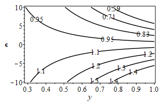
Figure 4.1: Variation of ϵ on the concentration profile
Figure 4.3 shows the effect of Schmidt number Sc on the concentration field. Schmidt number Sc is defined as the ratio momentum diffusivity (kinematic viscosity) and mass diffusivity. It is seen that the higher value of Schmidt number Sc reduces concentration. Figure 4.4 demonstrates the profiles of species concentration with various values of Prandtl number Pr. The prandtl number represents the ratio of momentum diffusivity to thermal diffusivity which justify the fact that an increase Pr causes decrease in concentration profiles.
Figure 4.5 depicts the effect of Schmidt number Sc on the velocity field. It is observed when molecules collide randomly, the momentum diffusivity parameter increases which increases the Schmidt number and result in velocity argumentation. Figure 4.6 demonstrates the profiles of velocity with Prandtl number Pr. The Prandtl number Pr which is defined as the ratio of momentum diffusivity to thermal diffusivity It is evident that velocity profile increases with augmentation in Prandtl number Pr. The influence of Grashof number on the temperature field is shown in Figure 5.7. If the thermal Grashof number prevail then the temperature distribution decreases but if the mass buoyancy dominates, temperature distribution increases. Figure 4.8 represent the buoyancy effect on the temperature distribution. Increase in buoyancy decreases temperature. The Reynolds number’s behavior on the temperature field is shown in Figure 4.9. The ratio of inertial forces to viscous forces is known as the Reynolds number. At decreasing Reynolds number levels, the fluid loses some of its viscosity. The viscous forces are subordinated to the inertial forces, increasing the fluid temperature. Figure 4.10 illustrate the effect of Schmidt number Sc on the temperature profile. An increase in Schmidt number Sc decreases the temperature profile. Figure 4.11 demonstrates the profiles of temperature with variation of Prandtl number Pr. The prandtl number is ratio of momentum diffusivity to thermal diffusivity which clarify the fact that an increase Pr causes decrease in temperature profiles.
Figure 4.2: Variation of π0 on the concentration profile
CONCLUSION
This research paper presents a comprehensive investigation into the stability of magnetohydrodynamic flow in channels occupied by porous media, considering modifications to the classical Orr-Sommerfeld analysis using the Darcy-Forchheimer model. The study contributes to the understanding of flow stability in complex porous media environments and lays the foundation for further research in this area. Insights gained from this study can inform the design and optimization of engineering systems involving MHD flows in porous media-filled channels.
The Modified Orr-Sommerfeld MHD Stability Flow in a Channel occupy by Porous Medium was investigated. The governing non-linear partial differential equations are solved separately to obtain the mean velocity, mean temperature and the mean concentration along with the oscillatory part of the velocity, temperature and concentration. From the computational results, the influences of various physical parameters such as on the profiles of velocity, temperature and species concentration are analyzed.
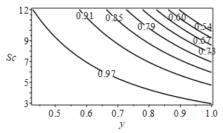
Figure 4.3: Variation of Sc on the concentration profile
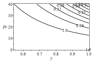
Figure 4.4: Variation of Pr on the concentration profile
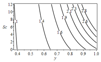
Figure 4.5: Effects of Sc on the velocity field
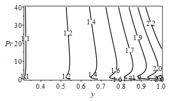
Figure 4.6: Effects of Pr on the velocity field.
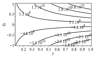
Figure 4.7: Effects of G on the temperature field.
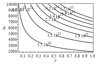
Figure 4.8: Effects of N on the temperature field
In general, particularly in our context of stability analysis, uniform contour lines typically refer to regions in parameter space where the behavior of the system remains consistent or stable. In summary, our results reveal:
Stable Regions: Contour lines that are uniform or nearly uniform across a region of parameter space indicate regions where the system’s behavior is stable. This means that small perturbations or changes in parameters within that region do not lead to significant deviations or instability in the system’s response. In this analysis where contour lines represent temperature velocity, temperature or concentration, uniform contours indicate that the system has reached momentum, thermal or species equilibrium.
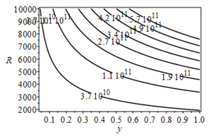
Figure 4.9: Effects of R on the temperature field.
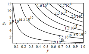
Figure 5.10: Effects of R on the temperature field
Robustness: Uniform contour lines suggest robustness of stability with respect to variations in parameters. A System designed with suggested parameters (as in our report) indicate that stability is maintained over a range of parameter values, which is often desirable in practical applications where parameters may vary.
Parameter Sensitivity: In this analysis, contour lines that are almost parallel and equally spaced, indicate that the field (velocity, temperature or concentration) being analyzed is not highly sensitive to changes in the independent variables within that region. In other words, small changes in the input variables do not significantly affect the output values. Conversely, in some cases, regions where contour lines are highly variable or non-uniform indicate parameter sensitivity and instability. In such regions, small changes in parameters can lead to significant changes in the system’s behavior, potentially resulting in instability or unpredictable responses.
Uniform Boundary Conditions: Uniform contour lines can also arise when boundary conditions, such as velocity, temperature or concentration at the boundaries of the system, are constant or vary smoothly.
Balanced Heat or Mass Transfer: Uniform contour lines also suggest regions where heat or mass transfer rates are balanced, meaning that the rates of heat or mass transfer into the region are approximately equal to the rates of heat or mass transfer out of that region.
Therefore, the result of this work will help to identify stable regions, assess parameter sensitivity, and understand the boundaries of stability within the system’s parameter space.
ACKNOWLEDGEMENT
We would like to express our sincere gratitude to the constructive feedback provided by the anonymous reviewers and the editorial team, which helped enhance the clarity and rigor of this manuscript.
CONFLICT OF INTEREST
The authors declare that there are no conflicts of interest regarding the publication of this manuscript.
REFERENCES
- Reynolds, O. (1883) An experimental investigation of the circumstances which determine whether the motion of water shall be direct or sinuous and the law of resistance in parallel channels. Phil. Trans. R. Soc. 174, 935–982. (doi:10.1098/rstl.1883.0029).
- Orr, W. MF (1907). The stability or instability of steady motions of a perfect liquid and of a viscous liquid, Proc. Roy. Irish Academy, A 27, 9-68, 69-138.
- Sommerfeld, A. (1908), Ein Beitrag zur hydrodynamischen Erklaerung der turbulenten Fluessigkeitsbewegungen, Proc. 4th International Congress of Mathematicians, Rome Vol III, 116-24.
- Hayat, T., Sajjada, R., Abbasc, Z., Sajidd, M and Hendie, A. A. (2011). “Radiation effects on MHD flow of Maxwell fluid in a channel with porous medium,” International Journal of Heat & Mass Transfer, 54, 854–862.
- Umavathi, J. C and Veershetty, S. (2012): Non-Darcy mixed convection in a vertical porous channel with boundary conditions of third kind. Transport in Porous Media, 95(1), 111-131.
- Krishnamurthy, M. R., Gireesha, B. J., Gorla, R.S.R. and B.C. Prasannakumara, B. C. (2016). Suspended Particle effect on slip flow and melting heat transfer of nanofluid over a stretching sheet embedded in a porous medium in the presence of nonlinear thermal radiation, J. Nanofluids 5, 502-510.
- Haider, F., Hayat, T and Alsaedi, A. (2021). Flow of hybrid nanofluid through Darcy-Forchheimer porous space with variable characteristics, Alexandria Engineering Journal, 60(3), 3047–3056.
- Okedoye, A. M (2013). Analytical Solution of MHD Free Convective Heat and Mass Transfer Flow in a Porous Medium. The Pacific Journal of Science, 14(2), 119-128.
- Ibrahim, S. Y. and Makinde, O. D. (2013). Chemically reacting MHD boundary layer flow of heat and mass transfer over a moving vertical plate with suction. Scientific Research and Essays, 5(19), 2875-2882.
- Hunegnaw, D. and Kishan, N. (2014). Unsteady MHD heat and mass transfer flow over stretching sheet in porous medium with variable properties considering viscous dissipation and chemical reaction. American Chemical Science Journal, 4(6), 901-917.
- Adesanya, S. O., Oluwadare, E. O., Falade, J. A., Makinde, O. D. (2015). Hydromagnetic natural convection flow between vertical parallel plates with time-periodic boundary conditions. J. Magn. Magn. Mater. 396, 295–303.
- Okedoye, A. M. (2015). Entropy generation in combined heat and mass transfer effect on MHD free convection flow past an oscillating plate. Journal of Mathematic Sans Science (JMS), 4(1), 1-12.
- Mabood, F., Ibrahim, S.M., Rashidi, M.M., Shadloo, M.S., and Lorenzini, G. (2016) Non-Uniform Heat Source/Sink and Soret Effects on MHD Non-Darcian Convective Flow past a Stretching Sheet in a Micropolar Fluid with Radiation, International Journal of Heat Mass Transfer, 93, 674–682. https://doi.org/10.1016/j.ijheatmasstransfer.2015.10.014 .
- Liu, HH. (2017). Generalization of Darcy’s Law: Non-Darcian Liquid Flow in Low-Permeability Media. In: Fluid Flow in the Subsurface. Theory and Applications of Transport in Porous Media, vol 28. Springer, Cham. https://doi.org/10.1007/978-3-319-43449-0_1
- Shehzad S. A., Abbasi, F. M., Hayat, T., Alsaedi, A. (2016). Catteneo-Christov heat flux transfer for Darcy-Forchheimer flow of an Oldroyd-B fluid with variable conductivity and non-linear convection. J Mol Lig; 224:274-8.
- Hayat T., Muhammad T., Al-Mezal, S., Liao, S. J. (2016). Darcy-Forchheimer flow with variable thermal conductivity and Catteneo-Christov heat flux. International Journal of Numerical Methods Heat Fluid Flow; 26: 2355-69.
- Gbadeyan, J. A and Opanuga, A. A. (2018). Inherent irreversibility analysis in a buoyancy induced magnetohydrodynamic couple stress fluid. Journal of Mathematics and Computer Science, 18, 411–422. doi: 10.22436/jmcs.018.04.03
- Abbas, Z., Naveed, M., Hussain, M and Salamat, N. (2020). Analysis of entropy generation for MHD flow of viscous fluid embedded in a vertical porous channel with thermal radiation. Alexandria Engineering Journal, 59, 3395–3405. https://doi.org/10.1016/j.aej.2020.0 5.019.
- Okedoye A. M and Salawu S. O. (2019): Effect of nonlinear radiative heat and mass transfer on MHD flow over a stretching surface with variable conductivity and viscosity, Journal of the Serbian Society for Computational Mechanics, 13(2), pp.87-104.
- Kumar, R. V. M. S. S. K. and Varma, S. V. K. (2018). “MHD boundary layer flow of nanofluid through a porous medium over a stretching sheet with variable wall thickness: using Cattaneo– Christov heat flux model, Journal of Deoretical and Applied Mechanics, 48(2), 72–92. DOI: 10.2478/jtam-2018-0011.
- Menni, Y, A. J. Chamakha, A. J. and A. Azzi, A. (2019). “Nanofluid transport in porous media: a review,” Special Topics & Reviews in Porous Media: An International Journal, 10 (1), 49-64. DOI:10.1615/SpecialTopicsRevPorousMedia.2018027168.
- Falana, A and Alao, A. A. (2019). Similarity Solution of Heat and Mass Transfer Flow of a Nanofluid across a Porous Plate in a Darcy-Forchheimer Flow. Current Journal of Applied Science and Technology 34(1).
- Sharma, R. P and S. R. Mishra, S. R. (2020). “Effect of higher order chemical reaction on magnetohydrodynamic micropolar fluid flow with internal heat source,” International Journal of Fluid Mechanics Research, 47(2) 121–134.
- Eid, M. R., Mahny, K. L and Al-Hossainy, A. F. (2021). Homogeneous-heterogeneous in the MHD flow of a non-Newtonian Prandtl fluid via a permeable linear horizontal expandable (shrinkable) surface. Surfaces and Interfaces 24, 101.
- Panya, A. L, Akeyemi, A.O and Okedoye, A. M. (2023): MHD Darcy-Forchheimer Slip Flow in a Porous Medium with Variable Thermo-Physical Properties. International Journal of Mechanical Technology. 10(2), (30-42), ISSN 2348-7593. DOI: https://doi.org/10.5281/zenodo.7646344.
- Abdul Hakeem, A. K., Vishnu Ganesh, N. and Ganga, B. (2014). Effect of heat radiation in a Walter’s liquid B fluid over a stretching sheet with non-uniform heat source/sink and elastic deformation, Journal of King Saud University – Engineering Sciences, Volume 26, Issue 2, 2014, Pages 168-175, ISSN 1018-3639, https://doi.org/10.1016/j.jksues.2013.05.006.
- Arunachalam, M and Rajappa, N. R. (1978). Forced convection in liquid metals with variable thermal conductivity and capacity. Acta Mech., 31, 25–31.
Chiam, T. C. (1998). Magnetohydrodynamic heat transfer over a non-isothermal stretching sheet. Acta Mech., 122, 169. - Aziz, A., Saddique, J. I. and Aziz, T. (2014). Steady boundary layer slip flow along with heat and mass transfer over a porous plate embedded in a porous medium. PLoS ONE, 9(12), e114544, doi: 10.1371/journal.pone.0114544