
Evaluation of Geology and Hydrochemistry of Nawfia-Agulu Axis of Anambra State, Southeastern Nigeria
- Okolo, C.M
- Korie, J.I.
- Madu, F.M
- Ifeanyichukwu, K.A
- 506-527
- Apr 23, 2024
- Mass Communication
Evaluation of Geology and Hydrochemistry of Nawfia-Agulu Axis of Anambra State, Southeastern Nigeria
Okolo, C.M, Korie, J.I., Madu, F.M and Ifeanyichukwu, K.A
Department of Geological Sciences, Nnamdi Azikiwe University, Awka
DOI: https://doi.org/10.51584/IJRIAS.2024.90346
Received: 12 March 2024; Accepted: 23 March 2024; Published: 22 April 2024
ABSTRACT
The investigation of the geological, hydrochemical, and engineering characteristics of the Nawfia – Agulu area was carried out. The study aimed at mapping the geology through field data collection, outcrop logging, and laboratory analysis. Consequently, eleven soil and ten water samples were collected and analyzed through particle size distribution test; Atterberg limits tests and hydrochemical analysis to provide insights into the lithology, sediment characteristics, and water quality. The results indicated the dominance of the Ameki/Nanka Formation and Imo Formation as the underlying geology of the study area. The grain sizes of the sand samples ranged from medium to coarse grained, moderately to poorly sorted, and strongly positive to positively-skewed. The depositional environment was nearshore/beach, influenced by nearshore waves and turbulent currents. Engineering properties highlighted the prevalence of uniformly to well-graded soil and moderately to highly plastic behavior, as indicated by the mean plasticity index (PI) value of 26%. These findings suggest potential challenges for infrastructural development in some parts of the area. The water quality indicated slightly acidic water. The physical parameters and the major ions were within the permissible limits of World Health Organization (WHO) and the Nigerian Standard for Drinking Water Quality (NSDWQ). However, elevated concentrations of heavy metals, including lead, chromium, mercury, iron, and cadmium, in water sources exceeded the respective permissible limits for drinking water indicating contamination/pollution. The dominant water type was Ca2+ – Mg2+– SO42- – Cl– and the dominant hydrochemical process was simple dissolution or mixing and ion-exchange.
Keywords: Water Quality, Hydrochemical Analysis, Grain size Analysis, Nanka Formation
INTRODUCTION
Geology gives information on the underlying lithologies and formations of an area. The nature and the characteristics of the rocks that outcrop in an area not only affect the engineering properties but also the chemistry, composition and quality of the water resources. The engineering properties of rock depend on the grain sizes of the particles, its plasticity limits, swelling potential and moisture contents to mention but a few. It has been variously asserted that the chemistry and the mineralogical properties of rock leave their signature on the constituent of both surface water and groundwater (Elango and Postman, 2005, Anakwuba et al., 2020, Okolo et al., 2023). Some parts of the study area have considerable water resources (Nawfia area) while some parts (Agulu area) has paucity of surface water making groundwater and rain water harvesting the only alternative sources. However, much less information is available on groundwater resources of the area. The occurrence of groundwater is dependent primarily on the geology. It is a significant controlling factor that influences surface water and groundwater composition and groundwater recharge (Niyazi et al., 2023). The hydrochemistry of aquifers with the geological variables indicate that changes in mineralogy and lithology obviously influence the chemical composition of water and its hydraulic properties (Omonona and Okogbue, 2016). The correlation of water chemistry with local geology indicates the hydrochemical processes responsible for the composition. The influence of geology on hydrochemistry underscores the importance of the study of geology with respect to the water chemistry of the study area (Chitsazan et al., 2017). Evaluation of hydrogeochemical properties of groundwater plays a significant role in defining the suitability of water resources for various uses (Tolera et al., 2020, Omonona and Okogbue, 2016). Suitability of water resources for drinking and other purposes is determined by its physical and chemical properties (Wali et al., 2020). Therefore, it is vital to understand aquifer hydrochemistry for better water resources management. It is worthy of note that engineering geology uses the knowledge of geological and geomorphological techniques to facilitate infrastructural planning and engineering constructions. Mapping of the geology and geomorphology to assess the geological suitability is fundamental to the processes mentioned. Geology plays an important role in the construction industry in terms of maintaining a healthy environment and in planning large scale infrastructural development.
However, it was observed that detailed geological, hydrochemical and engineering geological studies in the study area is limited. Therefore, the present study will undertake the assessment of the underlying geology, environment of deposition, hydrochemistry and engineering geology of the study area using various methods.
Location of the study area
The study area is within the Nawfia-Agulu axis area of Anambra State, Southeastern Nigeria. It lies between latitudes 6º 10′ 0″ N and 6º 12′ 0″ N and longitudes 7º 0′ 0″ E and 7º 5′ 0″ E (Fig. 1). The study area have neighboring towns, such as Enugwu-Agidi, Enugwu Ukwu, Umuokpu, and Amawbia, Adazi-Nnukwu, Nri, Neni, Mbaukwu and Nibo. The settlement pattern within the area is mostly dispersed, and the major occupations practiced by the indigenes of the area include; trading, farming, river and lateritic sand mining and palm wine tapping. The area is generally accessible by major roads such as the Amawbia – Enugu-Agidi Road, Agulu-Amawbia road, Nibo Nise-Adazi road and the Amawbia-Nawfia road. However, some areas are accessed via minor roads and footpaths. The area has an undulating topography which accounts for the numerous erosion disasters and gullies (Egboka & Okpoko, 1984) in different locations of the study area. The study area encompasses both perennial and seasonal streams. The stream systems exhibit a dendritic drainage pattern, indicating the loose and unconsolidated nature of the formations in the study area. The study area has two dominant climatic seasons – the rainy (wet) and dry seasons. The wet season typically commences in late March and persists until October and, on occasion, November. Conversely, the dry season prevails from November to March (Nnadi et al., 2019, Ejikeme et al., 2017). According to Ifeka and Akinbobola (2015), the total annual rainfall is estimated to range between 1520–2020mm, with September being the month with the highest rainfall, reaching a peak of approximately 2500mm. The average daily and annual temperatures in the area are 28 °C and 27 °C, respectively that could increase up to approximately 32 °C during the hot periods of the year, which typically occur in February, and reduce to approximately 23 °C in the rainy season. In December, the area experiences the onset of the harmattan season, distinguished by low humidity levels.
Geology of the Study area
The study area is situated within the Niger Delta basin (Nwajide, 2013) and is distinguished by a varied physiography featuring both elevated highlands and lower-lying lowlands. The geology of the study area is characterized by the presence of two dominant local geologic units: the Imo Shale (Paleocene) and the Ameki/Nanka Formation (Eocene) within the Niger Delta Basin. The Imo Formation, recognized as the earliest formation in the Cenozoic Niger Delta Basin, unconformably underlies the Ameki Formation of the Ameki Group (Petters, 1991). The Paleocene to Eocene age of the Imo Formation was established through the analysis of macro and microfossils, including dinoflagellate cysts and microspore assemblages (Reyment, 1965, Short and Stäuble, 1967, Adegoke et al., 1980, Arua, 1980). Reyment’s (1965) analysis reveals a diverse composition of geological materials in the Imo Formation, including blue-grey clays, black shallow marine shales interbedded with calcareous sandstone bands, marl, and limestone. Lateral variations, such as the Ebenebe, Igbaku, and Umuna Sandstones, were observed in some southeastern regions of Nigeria (Anyanwu and Arua, 1990).
Following the deposition of the Imo Formation, the Eocene regression phase led to the formation of the Ameki Group. The Ameki Group comprises conformable sandstone and shale, suggesting a consistent sedimentary environment during deposition. It includes the Ameki Formation, primarily composed of marine facies (Reyment, 1965), and the Nanka and Nsugbe Formations, characterized mainly by tidal facies (Nwajide, 1980). The Nsugbe Formation was the initial sedimentary sequence deposited, followed by the Nanka and Ameki Formations (Nwajide, 1980).
Hydrogeology and Hydrochemistry of the Study Area
The hydrogeological framework of the study area is shaped by the presence of the Imo and Nanka Formations consisting of a series of aquifers which are separated by aquitards, thereby forming a multi-aquifer system (Onwuemesi et al, 1990). Also, the sandstone members – Ebenebe and Umunna Sandstones within the weathered Imo Formation, play a role in supplying temporary groundwater to the region (Anizoba, et. al., 2020). These are the topmost groundwater units recharged directly by infiltration from precipitation and base flow (Nfor et al., 2007). Also, the Nanka Formation constitutes deep confined aquifers with depth to exploitable groundwater ranging from 75m to 350m (Nfor et al., 2007). The unconfined aquifer system is typically less than 20m – 60m deep. The water table is very close to the ground surface and is controlled by seasonal variation (Nfor et al., 2007).
In-depth studies conducted by (Ngwoke et al., 2015) show significant heavy metal contamination in the groundwater of Agulu area with concentrations of lead and arsenic above the WHO allowable threshold. Specifically, the hydrochemistry profile of the study area exhibits a notable prevalence of lead (Pb) and arsenic (Ar) in the groundwater. The identified heavy metal concentrations emphasize the need for a thorough assessment of water quality, considering the potential implications for both environmental and public health concerns.
METHODOLOGY
The geologic field mapping involved outcrop studied, observation of the sedimentary structures and measurement of beddings and their orientation. The samples collected during the mapping were soil, sand and water samples (surface and groundwater) (Fig.1). Disturbed soil and sand samples were collected from different beds to ensure a representative sample. The samples were package in polyethylene bags and taken to laboratory for analyses. Equally, water samples were collected with clean plastic bottles from surface water and groundwater sources. The plastic cans were rinsed with the water samples before collection of samples. For surface water the sample bottles were fully submerged before collecting the samples. However, for groundwater the water was allowed to discharge for about five minutes before collection to ensure freshwater from the aquifer was collected. The sample bottles were covered with the plastic bottle cover. All the samples were appropriately labelled before being taken to the laboratory for analysis according to APHA (2005) standard methods. Some of the water samples were preserved with few drops of dilute hydrochloric acid before being stored in a container containing ice and taken to the laboratory. It is worthy to note that some water quality parameters such as pH, turbidity and electrical conductivity were tested in the field with a multi-parameter meter. The results were compared with WHO standard (2011) and NSDWQ, (2015).
The soil samples were subjected to Atterberg limits tests (plastic and liquid limit tests), while the sand samples were used for particle size distribution (PSD) analysis according to BS (1990) BS-1377 analytical methods. The Atterberg limit test was carried out to measure the consistency limits of fine-grained soils as it transits from one state of plasticity to another on the absorption of water. From the results the degree of plasticity of a given soil was inferred, and their suitability for engineering construction materials determined. The plasticity index of soil is the numerical difference between the liquid limit and plastic limit (PI = LL – PL). It is a direct indicator of how plastic a soil sample is.
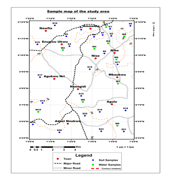
Fig.1: Map of the study area and samples location points
Particle Size Distribution (PSD) Analysis
The Particle Size Distribution (PSD) or grain size analysis is widely used in the classification of sands. The data obtained from the PSD analysis were used to compute the Median (M1), Mean grain size (M2), Standard Deviation (SD), Skewness (SK), and Kurtosis (K) using Folks and Ward (1957) method. The analysis of sediment grain size distribution provides valuable information about prevailing energy and hydrodynamic conditions during deposition. Mean size (M), standard deviation (ø), skewness (SK), and kurtosis (K) results were used to analyze grain size distribution, following Folk and Ward’s (1957) method as recommended by Sahu (1964). The average grain size, expressed as Phi (φ) = −log2 x D (D: size in mm), indicates energetic conditions during deposition, as observed by Sahu, (1964). Sorting, measured by the standard deviation from the mean, reflects the uniformity of the particle size distribution and is influenced by fluctuations in the energy and hydrodynamic conditions governing the deposition medium. Skewness, which measures the degree of asymmetry in the distribution, indicate the presence of a coarser (negative) or finer (positive) tail, revealing the mixing of sub-populations within the sediment. Finally, kurtosis results were used to evaluate the sorting of the tail, relative to the center of the curve. A Leptokurtic distribution indicates better sorting of the tail, whereas a Platykurtic distribution suggests poor sorting while a Mesokurtic distribution indicates uniform sorting between the tail and central part of the curve.
Coefficient of Uniformity (Cu) and Coefficient of Curvature (Cv)
These parameters were estimated using the gradation curve obtained through sieve analysis according to Murthy (2003) to identify grading of the soils.
Environmental Discrimination of Sand Sample
Sahu (1964) method was employed to differentiate the different environments and mediums of deposition. This method is based on the fact that each environment of deposition is characterized by a particular energy conditions reflected by the grain size distribution of sediments. The discriminate functions (Y1, Y2, Y3, and Y4) were applied to the sand samples for environmental analysis.
a. For discrimination between the Aeolian process and Littoral (intertidal) environments, the discriminate function in equation 1 was used
Y1 = -3.5688M + 3.7016ծ2 – 2.0766Sk + 3.1135K 1
Where;
- M = Mean grain size
- ծ = Inclusive graphic standard deviation (sorting)
- Sk = Skewness
- K =Graphic kurtosis,
- When Y1 is less than -2.7411 (Aeolian deposit is indicated)
- When Y1 is greater than -2.7411 (Littoral (tide) deposit is suspected).
b. For discrimination between the beach (back shore) and shallow agitated marine (subtidal) environment, the discriminate function used is given in equation 2.
Y2 = 15.6534M + 65.7091ծ2 + 18.1071Sk + 18.5043K 2
- When Y2 is less than 65.3650 (beach environment is suggested).
- When Y2 is greater than 65.3650 (shallow agitated marine environment (subtidal) is likely).
c. For the discrimination between shallow marine and fluvial environments, the discriminate function employed is stated in equation 3
Y3 = 0.2852M – 8.7604ծ2 – 4.89325Sk + 0.0482K 3
- When Y3 is less than -7.419 (the sample is identified as a fluvial (deltaic) deposit).
- When Y3 is greater than -7.419 (it is identified as shallow marine sand).
RESULTS AND DISCUSSIONS
Geologic field mapping and outcrop studies.
During the geologic field mapping of the study area, some of the outcrop exposures at different locations were studied and represented in Figs. 2, 3 and 4, and Table 5. The outcrop at location 4 was an erosional exposure. Three distinct strata were observed composing of a lateritic top, fine to coarse grained sand with ferruginized sandstone bed and the base is made up of dark grey shale (Fig. 2). Location 4 is Umukwa Gully with description as follows-
- Depth: 3.23 meters deep.
- Three distinct layers and brown lateritic covering (1.85m) grades into the second layer.
- The first layer is more consolidated and finer, with coarse grained Ironstone. It is poorly sorted with a thickness of 70cm.
- The second layer is an ironstone bed of 60cm thick, very coarse–grained and poorly sorted with strike direction 096º, Dip direction: 82º and Dip amount: 6º
- The third layer is a dark grey shale bed (Fig.2).
The outcrop at location 8 is an abandoned quarry site exposure (Fig. 3). The lithologic log indicates a lateritic top layer and five other distinct beds with variable colours. The colour can be attributed to the oxidation of iron present in the formation. The individual beds were sand with grains, shapes and sizes ranging from angular to rounded and fine to medium respectively. The lithologic log prepared from cuttings from a borehole at location 7 is shown in Fig. 4. A top lateritic cover was distinct with five other beds comprising sand fine to coarse grained and shale. The descriptions for all the locations were tabulated in Table 5.
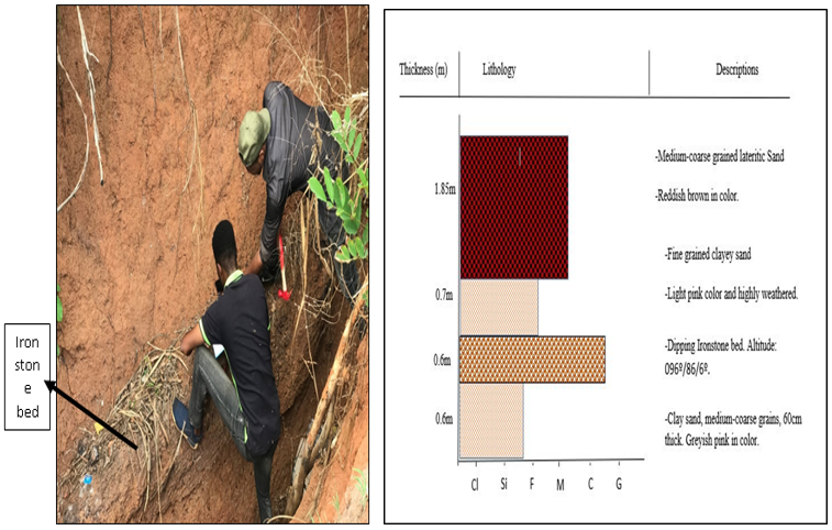
Fig. 2: Outcrop exposure and lithologic log at Umukwa Gully (location 4).
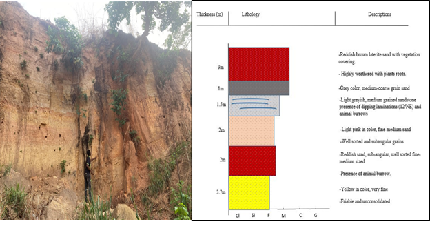
Fig. 3: Sandstone exposure and lithologic log of the outcrop exposure at location 8
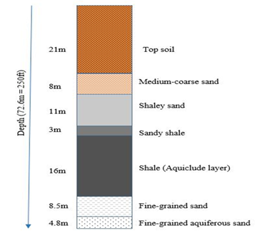
Fig.4: Borehole log made with cutting from newly constructed borehole at location 7
Table 5: Summary of outcrop description and studies
| Location No. | Latitude (North) | Longitude (East) | Elevation (m) | (Strike/dip/dip amount) | Lithology | Remark |
| 1 | 6º 13′ 17″ N | 7º 0′ 8″ E | 99 | – | Sandstone | Ezimezi Gully erosion site |
| 2 | 6º 11′ 52″ N | 7º 0′ 8″ E | 103 | – | Sandstone | Ovia Stream Channel |
| 3 | 6º 10′ 47″ N | 7º 1′ 35″ E | 113 | – | Shale | Ngene Ocha River channel |
| 4 | 6º 11′ 5″ N | 7º 1′ 20″ E | 94 | 092º/82º/6º | Sandstone (Ironstone beds) | Umukwa Gully |
| 5 | 6º 11′ 18″ N | 7º 3′ 34″ E | 91 | – | Sandstone, Clay | Along Amawbia-Nibo Rd |
| 6 | 6º 11′ 19″ N | 7º 03′ 36″ E | 91 | Dip amount = 12º | Sandstone | Along Amawbia-Nibo Rd |
| 7 | 6º 10′ 10″ N | 7º 03′ 49″ E | 147.5 | – | Sandstone, Shale | Borehole log. |
| 8 | 6º 11′ 58″ N | 7º 05′ 00″ E | 108 | – | Sandstone | Abandoned Excavation site along Nawfia-Agulu Rd |
| 9 | 6º 12′ 0″ N | 7º 1′ 16″ E | 129 | – | Sandstone | Excavation site Along Amawbia-Umuokpu Timber Market |
| 10 | 6° 09’ 24” N | 7° 04’ 11” E | 85 | – | Shale | Obini River channel, Nibo |
| 11 | 6° 08’ 16” N | 7° 04’ 29” E | 102 | – | Shale | Nora River channel, Mbaukwu |
| 12 | 6° 07’ 19” N | 7° 02’ 39” E | 127 | – | Shale | Idemili Omelagha River Channel, Agulu |
| 13 | 6° 07’ 24” N | 7° 02’ 33” E | 120 | – | Sandstone | Umuifite Gully erosion site, Agulu |
| 14 | 6° 04’ 58” N | 7° 05’ 17” E | 120 | – | Sandstone | Awgbu Gully Erosion site, Agulu |
| 15 | 6° 07’ 09” N | 7° 00’ 49” E | 113 | – | Sandstone | Adazi Nnukwu, Gully Erosion, Agulu |
| 16 | 6° 05’ 56” N | 7° 00’ 03” E | 207 | – | Sandstone, Shale | Borehole log at Neni |
| 17 | 6° 09’ 06” N | 7° 02’ 03” E | 138 | – | Sandstone, Shale | Borehole log at Agukwu Nri |
| 18 | 6° 09’ 08” N | 7° 01’ 13” E | 108 | – | Shale | Onu-Ngene River Channel, Nri |
| 19 | 6° 09’ 56” N | 7° 00’ 37” E | 197 | Dip amount = 6° | Sandstone (Ironstone) | Saraphina Hill, Enugwu-ukwu |
Geology of the study area.
The following deductions were made from the outcrop studies. It revealed that two characteristics dominant lithologies sandstone and shale (Table 5) underlie the study area. The sandstones were characteristics of the Ameki/Nanka Formation and the shale depicts the Imo Formation. The shale outcrops in the central and peripheral regions of the study area and it is overlain by the sand (Fig. 5).
Sedimentological, Textural and Depositional Analyses.
To further understand the lithologies in the study area the standard guidelines of the Unified Soil Classification System (USCS), and the Particle Size Distribution (PSD) analysis were employed. Two sets of particle size distribution curves were constructed for all the twenty-three (23) samples. The results of the Particle Size Distribution analysis for the all the samples were provided in Table 6.
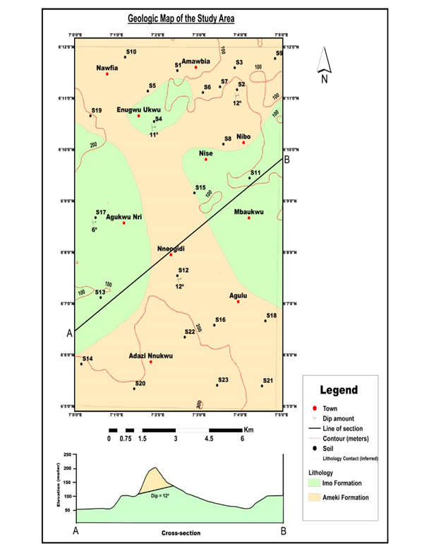
Fig. 5: Geologic map of the study area
Table 6: Result of some calculated sedimentological parameters from PSD analysis (according to Folk and Ward, 1957 modified)
| Sample
No. |
Mean | Remark | Standard deviation | Remarks | Skewness | Remarks | Kurtosis | Remarks |
| Sample 1 | 1.55 | Medium sand | 1.28 | Poorly sorted | 0.03 | Symmetrical | 1.16 | Leptokurtic |
| Sample 2 | 1.37 | Medium sand | 1.40 | Poorly sorted | 0.03 | Symmetrical | 0.86 | Platykurtic |
| Sample 3 | 1.36 | Medium sand | 1.43 | Poorly sorted | -0.14 | Positively (finely) skewed | 0.78 | Platykurtic |
| Sample 4 | 1.82 | Medium sand | 1.81 | Very poorly sorted | -0.29 | Positively (finely) skewed | 0.72 | Platykurtic |
| Sample 5 | 1.22 | Medium sand | 1.43 | Poorly sorted | 0.04 | Symmetrical | 0.77 | Platykurtic |
| Sample 6 | 0.45 | Coarse sand | 1.04 | Moderately sorted | -0.17 | Positively (finely) skewed | 1.28 | Leptokurtic |
| Sample 7 | 1.34 | Medium sand | 0.67 | Moderately sorted | 0.33 | Very positively skewed | 1.28 | Leptokurtic |
| Sample 8 | 0.48 | Coarse sand | 1.37 | Poorly sorted | 0.39 | Very positively skewed | 1.49 | Leptokurtic |
| Sample 9 | 1.78 | Medium sand | 0.97 | Moderately sorted | 0.39 | Very positively skewed | 1.36 | Leptokurtic |
| Sample 10 | 0.48 | Coarse Sand | 1.04 | Moderately sorted | 0.12 | Positively skewed | 0.94 | Mesokurtic |
| Sample 11 | 2.62 | Fine sand | 1.14 | Poorly sorted | -0.36 | Very negatively skewed | 1.45 | Leptokurtic |
| Sample 12 | 1.30 | Medium Sand | 1.29 | Poorly Sorted | 0.05 | Symmetrical | 1.16 | Leptokurtic |
| Sample 13 | 1.69 | Medium Sand | 1.05 | Poorly Sorted | -0.13 | Negatively Skewed | 1.44 | Leptokurtic |
| Sample 14 | 0.95 | Coarse Sand | 0.93 | Moderately Sorted | -0.10 | Symmetrical | 1.21 | Leptokurtic |
| Sample 15 | 0.65 | Coarse Sand | 0.68 | Moderately Sorted | -0.47 | Very Negatively Skewed | 0.83 | Platykurtic |
| Sample 16 | 2.62 | Fine Sand | 1.41 | Poorly Sorted | -0.31 | Very Negatively Skewed | 1.43 | Leptokurtic |
| Sample 17 | 1.05 | Medium Sand | 1.22 | Poorly Sorted | 0.00 | Symmetrical | 0.82 | Platykurtic |
| Sample 18 | 0.49 | Coarse Sand | 0.77 | Moderately Sorted | -0.18 | Negatively Skewed | 0.68 | Platykurtic |
| Sample 19 | 1.32 | Medium Sand | 0.69 | Moderately Sorted | -0.08 | Symmetrical | 1.42 | Leptokurtic |
| Sample 20 | 2.16 | Fine Sand | 1.12 | Poorly Sorted | 0.45 | Very Positively Skewed | 0.48 | Very Platykurtic |
| Sample 21 | 1.30 | Medium sand | 0.44 | Well Sorted | 0.28 | Very Positively Skewed | 0.79 | Platykurtic |
| Sample 22 | -0.15 | Very Coarse Sand | 1.77 | Poorly Sorted | 0.05 | Symmetrical | 0.86 | Platykurtic |
| Sample 23 | 1.99 | Medium Sand | 1.39 | Poorly Sorted | -0.34 | Very Negatively Skewed | 1.05 | Mesokurtic |
Textural analysis reveals that the sediments were poorly (47.8%) to moderately (52.2%) sorted. The sediments were very positively (39.1%), very negatively (26%) skewed and symmetrical (34.9%). Further it was observed that the sediments were platykurtic (43.5%), leptokurtic (47.8%) and mesokurtic (8.7%). These observations suggest a mixed depositional environments and processes indicative of a prograding deltaic system. Such a system is usually characterized by good sediment supply to the coast by rivers and distributed along the coastline by waves and currents (Posamentier and Allen, 1999). The mean grain size ranges from 0.45 to 2.62mm indicative of medium to coarse grained sandstone. However, employing Sahu (1964) approach to perform linear discriminate analysis based on the three functions (Y1, Y2, and Y3) on the soil samples, provided additional insights into the depositional setting and the agent responsible for deposition. Y1 and Y2 functions indicate littoral processes, beach, and shallow agitated marine environments (Table 7) while Y3 function revealed that 72.73% of the samples were fluvial deposits, while the remaining 27.27% indicate shallow marine deposits. The combination of littoral processes and beach environment suggests sediments deposited in a nearshore environment, where waves and currents have significantly influenced their transport, deposition, and sorting. The present result is similar to the report of Allen and Posamentier (1993). Additionally, the shallow agitated marine environments observed were indicative of deposition in a shallow, wave-dominated marine environment, which aligns with the observations of poor to moderate grain sorting as noted by Nichols (2009) and Nwajide (2013). Therefore, depositional environment was characterized by littoral processes, including high-energy tidal waves, turbulent current actions, and periodic fluvial sediment influxes from nearby river system. The result can be summarized as a marginal marine environment with low to moderate depositional energy.
Table 7: Summary of values of linear discriminate functions for all samples.
| Samples | Y1 | Y2 | Y3 |
| Sample 1 | 4.41
Littoral (tidal) deposit |
153.93
Shallow agitated marine environment. |
-14.40
Fluvial deposit |
| Sample 2 | 5.27
Littoral (tidal) deposit |
166.69
Shallow agitated marine environment. |
-17.28
Fluvial deposit |
| Sample 3 | 5.72
Littoral (tidal) deposit |
167.56
Shallow agitated marine environment. |
-14.95
Fluvial deposit |
| Sample 4 | 8.86
Littoral (tidal) deposit |
251.83
Shallow agitated marine environment. |
-22.90
Fluvial deposit |
| Sample 5 | 5.79
Littoral (tidal) deposit |
168.44
Shallow agitated marine environment. |
-18.25
Fluvial deposit |
| Sample 6 | 6.83
Littoral (tidal) deposit |
98.72
Shallow agitated marine environment. |
-6.21
Shallow marine sand |
| Sample 7 | 0.46
Littoral (tidal) deposit |
80.13
Shallow agitated marine environment. |
-9.46
Fluvial deposit |
| Sample 8 | 9.17
Littoral (tidal) deposit |
165.48
Shallow agitated marine environment. |
-23.30
Fluvial deposit |
| Sample 9 | 0.93
Littoral (tidal) deposit |
121.92
Shallow agitated marine environment. |
-14.73
Fluvial deposit |
| Sample 10 | 5.07
Littoral (tidal) deposit |
98.15
Shallow agitated marine environment. |
-11.47
Fluvial deposit |
| Sample 11 | 1.28
Littoral (tidal) deposit |
146.72
Shallow agitated marine environment. |
-4.05
Shallow marine sand |
| Sample 12 | 5.03
Beach environment. |
152.07
Shallow agitated marine environment. |
-14.40
Fluvial deposit |
| Sample 13 | 2.80
Beach environment. |
23.19
Shallow agitated marine environment. |
-8.47
Fluvial deposit |
| Sample 14 | 3.79
Beach environment. |
92.28
Shallow agitated marine environment. |
-6.76
Shallow marine sand |
| Sample 15 | 2.95
Beach environment. |
47.41
Beach deposition |
-1.53
Shallow marine sand |
| Sample 16 | 3.10
Beach environment. |
192.50
Shallow agitated marine environment. |
-15.08
Fluvial deposit |
| Sample 17 | 4.32
Beach environment. |
129.41
Shallow agitated marine environment. |
-12.70
Fluvial deposit |
| Sample 18 | 2.94
Beach environment. |
55.95
Beach deposition |
-4.14
Sh 1`Q9hallow marine sand |
| Sample 19 | 1.64
Beach environment. |
76.77
Shallow agitated marine environment. |
-3.33
Shallow marine sand |
| Sample 20 | -2.51
Beach environment. |
133.27
Shallow agitated marine environment. |
-12.55
Fluvial deposit |
| Sample 21 | -2.04
Beach environment. |
52.76
Beach deposition |
-3.33
Shallow marine sand |
| Sample 22 | 14.71
Beach environment. |
220.33
Shallow agitated marine environment. |
-27.69
Fluvial deposit |
| Sample 23 | 4.03
Beach environment. |
171.38
Shallow agitated marine environment. |
-14.64
Fluvial deposit |
Engineering properties of sand and soil in the study area
The results of the Particle Size Distribution (Table 6) reveal that standard deviation range from 0.67 to 1.81 with a mean of 1.23. The soils were classified using the Unified Soil Classification system (USCS, 1986). The liquid limit of the soil was determined as the moisture content corresponding to the 25th blow. Comprehensive information on all the samples were summarized in Table 9. The coefficient of uniformity ranged from 1.89 to 15.96 with a mean value of 1.56. However, the coefficient of curvature ranged from 0.57 to 4.41 with a mean value of 1.73. The coefficient of uniformity ranked the soils as uniformly graded (56.5%) to well- graded (43.5%) though the coefficient of curvature ranked the soils as well grade with the exception of sample 10 which was gap-graded. The gradation of soil affects engineering properties such as shear strength and compressibility. Well-graded soils have more interlocking between particles and thus a higher friction angle, than uniformly graded soils. The compressibility of well-graded soil is almost none existent while that of uniformly grade soil is high. Hence, permeability is higher in uniformly graded soil making well-graded soil more suitable for engineering construction.
Atterberg limits were not only used to identify the soils classification but also for empirical correlations to determine some other engineering properties. The swelling potential of the soil samples ranged from medium to high (Table 9), which indicated that the soil may expand significantly when it comes into contact with water. This action can cause damage to the foundation and pavement structures over time. Drainage systems need suitable soil to support engineering structures such as houses and pavements. The swelling potential of the soil samples ranges from medium to high. It can to be designed to control the water content of the soil and prevent excessive swelling.
In summary, the well-graded soils possess desirable characteristics such as good drainage properties, low compressibility, and high shear strength, which make them suitable for engineering applications such as shallow and deep foundations, embankments and pavements. The high plasticity and swelling potential of some samples may limit their suitability for certain engineering applications, particularly for higher loads and taller structures.
Table 8: Summary statistics of grain size distribution indices coefficient of uniformity (Cu) and coefficient of curvature (Cc) (Murthy, 2003)
| Sample Number | Coefficient of uniformity | Remarks | Coefficient of curvature | Remarks |
| Sample 1 | 3.99 | Uniformly graded | 1.21 | Well graded |
| Sample 2 | 6.57 | Well graded | 1.56 | Well graded |
| Sample 3 | 6.39 | Well graded | 1.28 | Well graded |
| Sample 4 | 6.59 | Well graded | 0.57 | Well graded |
| Sample 5 | 7.76 | Well graded | 1.58 | Well graded |
| Sample 6 | 12.12 | Well graded | 3.75 | Well graded |
| Sample 7 | 3.17 | Uniformly graded | 1.57 | Well graded |
| Sample 8 | 15.96 | Well graded | 4.41 | Well graded |
| Sample 9 | 2.62 | Uniformly graded | 1.12 | Well graded |
| Sample 10 | 3.81 | Uniformly graded | 0.87 | Gap graded |
| Sample 11 | 2.62 | Uniformly graded | 1.12 | Well graded |
| Sample 12 | 3.75 | Well graded | 1.11 | Well graded |
| Sample 13 | 2.52 | Uniform graded | 1.04 | Well graded |
| Sample 14 | 2.13 | Uniform graded | 1.04 | Well graded |
| Sample 15 | 1.89 | Uniform graded | 1.29 | Well graded |
| Sample 16 | 2.43 | Uniform graded | 0.84 | Well graded |
| Sample 17 | 3.66 | Well graded | 0.99 | Well graded |
| Sample 18 | 2.90 | Uniform graded | 0.81 | Well graded |
| Sample 19 | 1.77 | Uniform graded | 0.95 | Well graded |
| Sample 20 | 4.84 | Well graded | 0.76 | Well graded |
| Sample 21 | 1.73 | Uniform graded | 0.97 | Well graded |
| Sample 22 | 7.90 | Well graded | 0.91 | Well graded |
| Sample 23 | 2.83 | Uniform graded | 0.82 | Well graded |
| Mean | 6.51 | – | 1.73 | – |
Table 9: Summary statistics of the Liquid limit and Plastic limit results for samples (1-8).
| Sample No. | Liquid Limit (%) | Plastic Limit (%) | Plasticity Index (%) | Remark | Swelling potential |
| Sample 1 | 53 | 36 | 17 | High plastic | High |
| Sample 2 | 35 | 17 | 18 | Moderately plastic | Medium |
| Sample 3 | 37 | 19 | 18 | Moderately plastic | Medium |
| Sample 4 | 52 | 17 | 35 | High plasticity | High |
| Sample 5 | 54 | 12 | 42 | Very High plasticity | High |
| Sample 6 | 35 | 20 | 15 | Moderately plastic | Medium |
| Sample 7 | 47 | 19 | 28 | High plasticity | High |
| Sample 8 | 50 | 16 | 34 | High plasticity | High |
Hydrochemistry
The physical and chemical aspects of water quality were considered. The concentration of analyzed parameters were compared with the WHO and NSDWQ to determine the level of risk. The results of the water analysis were summarized in Table 10 for surface water and Table 11 for groundwater.
Surface water
The concentrations for TDS, electrical conductivity and turbidity ranged from 11 – 42mg/l, 34 – 82.4µS/cm and 1.30 -1.50 NTU respectively. The concentrations were within the guideline values. The pH of surface water samples ranged from 6.24 – 6.42 indicating slightly acidic water. It was observed that 80% of the surface water samples did not meet the permissible limit of the guidelines. The major cations and anions did not exceed the permissible limit of the guideline values. However, the concentration of chloride 120 – 167mg/l and sulphate 67.02 – 163.67mg/l were slightly elevated. This could be as a result of input from industrial and domestic sewage, a similar observation was made by (Okolo et al., 2018, Madu, et al., 2022). The distribution of the physical parameters and major ions were shown in Fig.8. Also, the distribution of the heavy metals was shown in Fig.9. The heavy metals analyzed include chromium, cadmium, mercury, lead and iron. Chromium concentration ranges from 0.037 to 0.093 ppm, with a mean value of 0.061 ppm, exceeding the permissible limits set by both the WHO and NSDWQ. The concentrations of mercury (0.005 to 0.009 ppm with a mean value of 0.016 ppm), cadmium (0.003 to 0.022 ppm, with a mean value of 0.014 ppm), lead (0.052 – 0.089ppm) and iron (0.209 – 0.344ppm) exceed the guidelines permissible limits. The presence of the heavy metals in the surface water has been variously attributed to anthropogenic pollution (Okolo et al., 2020). The present is similar to that reported by Ngwoke et al. (2015). The risk of heavy metals exceeding the permissible limits stems from their potential in deterioration of public health. The metals have been implicated in health-related disorders such as kidney diseases, bone defects, high blood pressure, neurological defects and diabetes (Mitra et. al., 2022). Elevated concentration of iron in the study area has been previously reported (Okolo et al., 2020, Okolo et al., 2024) which they attributed to mostly geogenic input. The danger of high concentration of iron was related to deposition of scales in boiler and kitchen utensils, and addition of bitter taste to the water.
Table 10: Concentration of physical and chemical parameters in the surface water sample.
| Samples | NS1 | NS2 | NS3 | AS1 | AS2 | AS3 | Mean | WHO | NSDWQ |
| Chromium (ppm) | 0.060 | 0.093 | 0.044 | 0.085 | 0.049 | 0.037 | 0.061 | 0.05 | 0.05 |
| Mercury (ppm) | 0.009 | 0.005 | 0.009 | 0.044 | 0.012 | 0.019 | 0.016 | 0.006 | 0.006 |
| Cadmium (ppm) | 0.020 | 0.022 | 0.010 | 0.008 | 0.003 | 0.019 | 0.014 | 0.003 | 0.003 |
| Lead (ppm) | 0.078 | 0.052 | 0.067 | 0.089 | 0.067 | 0.079 | 0.072 | 0.1 | 0.01 |
| Iron (ppm) | 0.322 | 0.493 | 0.209 | 0.344 | 0.279 | 0.0.329 | 0.329 | 0.3 | 0.5 |
| Calcium (ppm) | 9.020 | 5.022 | 4.010 | 4.008 | 4.003 | 7.019 | 5.514 | 75 | – |
| Magnesium (ppm) | 3.022 | 3.892 | 4.092 | 2.228 | 3.056 | 5.019 | 3.552 | 50 | 0.2 |
| Sodium (ppm) | 4.028 | 5.278 | 6.098 | 4.338 | 4.956 | 5.289 | 4.998 | 200 | – |
| Potassium (ppm) | 4.922 | 5.433 | 7.289 | 6.458 | 7.223 | 4.939 | 6.044 | – | – |
| Bicarbonate (mg/l) | 5.00 | 2.50 | 5.00 | 7.50 | 2.50 | 2.50 | 4.17 | 500 | 100 |
| Chloride (mg/l) | 167.00 | 160.00 | 130.00 | 120.00 | 147.00 | 137.00 | 143.5 | 250 | 250 |
| Nitrate (mg/l) | 8.26 | 4.35 | 8.60 | 5.76 | 5.83 | 4.21 | 6.17 | 50 | 50 |
| Sulphate (mg/l) | 145.26 | 67.02 | 160.25 | 99.17 | 87.65 | 163.67 | 120.50 | 500 | 200 |
| pH | 6.32 | 6.37 | 6.42 | 6.35 | 6.50 | 6.24 | 6.37 | 6.5-8.5 | 6.5-8.5 |
| TDS (mg/l) | 80.00 | 46.00 | 49.00 | 36.00 | 27.00 | 27.00 | 44.167 | 1,000 | 500 |
| Conductivity (µS/cm) | 182.70 | 94.20 | 104.80 | 67.40 | 34.70 | 39.80 | 87.267 | 2,000 | 1,000 |
| Turbidity (NTU) | 1.10 | 1.20 | 1.00 | 1.80 | 1.30 | 1.20 | 1.267 | 5 | 5 |
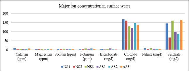
Fig. 8: The distribution of major ions in surface water
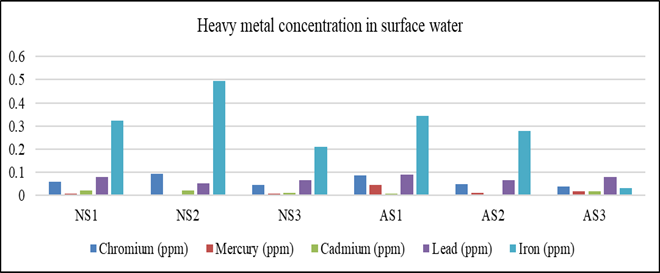
Fig. 9: The distribution of heavy metals concentration in the surface water.
Groundwater
The result of the physical parameters turbidity (1.30 -1.50NTU), electrical conductivity (34.00 -82.40µS/cm) and total dissolved solids (11.00 – 42.00mg/l) were within the guideline values. However, the pH of groundwater ranges from 6.10 – 6.58 indicating slightly acidic water. The pH of groundwater has been known to be slightly acidic because of the decay of organic matter, presence of carbon-dioxide and the reaction between carbon-dioxide and water (Freeze and Cherry, 1979). The major ion concentrations were within the permissible limits of WHO and NSDWQ. The heavy metals in groundwater iron (0.077 -0.452ppm), chromium (0.020 -0.056ppm), cadmium (0 – 0.19ppm), mercury (0.007 -0.027ppm) and lead (0.045 – 0.109ppm) exceed the guideline values in some samples. The presence of heavy metals in ground water is an indication of anthropogenic contamination/pollution. The physical properties and the major ions in both groundwater and surface water indicate that the water sources are good for drinking purposes. However, the elevated concentrations of heavy metals call for caution in the use of the water sources for drinking purposes. There is therefore need for pre-use treatment. The distribution of the physicochemical parameters was shown in Figs. 10 and 11.
Table 11: Concentration of physical and chemical parameters in groundwater sample.
| Samples | NG4 | NG5 | AG4 | AG5 | Mean | WHO | NSDWQ |
| Chromium (ppm) | 0.028 | 0.020 | 0.056 | 0.019 | 0.031 | 0.05 | 0.01 |
| Mercury (ppm) | 0.010 | 0.027 | 0.010 | 0.007 | 0.014 | 0.006 | 0.006 |
| Cadmium (ppm) | 0.019 | 0.006 | 0.006 | 0.00 | 0.008 | 0.005 | 0.005 |
| Lead (ppm) | 0.049 | 0.068 | 0.109 | 0.045 | 0.068 | 0.01 | 0.01 |
| Iron (ppm) | 0.229 | 0.168 | 0.452 | 0.077 | 0.232 | 0.3 | 0.5 |
| Calcium (ppm) | 5.019 | 7.006 | 6.006 | 9.043 | 6.769 | 75 | – |
| Magnesium (ppm) | 3.493 | 2.982 | 4.336 | 4.092 | 3.726 | 50 | 0.2 |
| Sodium (ppm) | 4.228 | 6.783 | 6.094 | 4.899 | 5.501 | 200 | 200 |
| Potassium (ppm) | 5.034 | 4.289 | 3.926 | 8.594 | 5.461 | – | – |
| Bicarbonate (mg/l) | 5.00 | 5.00 | 5.00 | 7.50 | 5.625 | 500 | 100 |
| Chloride (mg/l) | 115.00 | 125.00 | 133.00 | 155.00 | 132.00 | 250 | 250 |
| Nitrate (mg/l) | 4.41 | 4.28 | 4.28 | 4.07 | 4.26 | 50 | 50 |
| Sulphate (mg/l) | 88.47 | 79.26 | 67.08 | 105.76 | 85.14 | 500 | 200 |
| pH | 6.58 | 6.10 | 6.26 | 6.25 | 6.298 | 6.5 – 8.5 | 6.5 – 8.5 |
| TDS (mg/l) | 42.00 | 11.00 | 40.00 | 40.00 | 33.25 | 1,000 | 500 |
| Conductivity (µS/cm) | 82.40 | 34.00 | 74.20 | 79.40 | 67.50 | 1,000 | 5000 |
| Turbidity (NTU) | 1.40 | 1.30 | 1.50 | 1.40 | 1.40 | 5 | 5 |
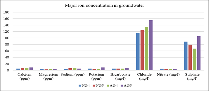
Fig. 10: Major ion concentration in Groundwater
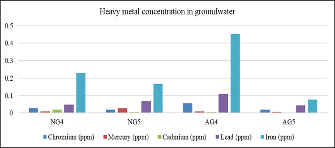
Fig. 11: Heavy metal concentration in Groundwater.
Hydrochemical processes
The hydrochemical processes were studied using the major ions which were used to plot the Piper (1944) and the Durov (1948) diagrams, Figs. 12 and 13 respectively. The analysis of the Piper plot revealed mixing of water in the cation domain showing no dominant cation. In addition, the anion domain indicates chloride as the dominant anion though the points fall on the sulphate line indicating its influence on the water chemistry. According to Back and Hanshaw (1965) classification the dominant facies were Ca2++Mg2+ > Na++K+ and the SO42-+Cl– > CO32-+HCO3–. The dominant water type was the Ca2+-Mg2+-Cl–-SO42- type. It is a water type in which the alkaline earth metals (Ca2+ and Mg2+) dominate over the alkali metal (Na+ and K+) while the strong acids (Cl– and SO42-) dominate over the weak acids (CO32- and HCO3–). The water type is associated with permanent hardness. To further understand the water chemistry, the Durov diagram (Fig. 13) was employed using the classification proposed by Lloyd and Heatcoat (1985). The plot indicated that 80% the plotted points were in field 5 indicating simple dissolution or mixing while the other 20% were located in domain 4 indicating ion exchange processes. The trend indicates recent fresh water exhibiting simple dissolution or mixing and ion exchange. Therefore, the dominant hydrochemical processes were dissolution of the underlying geologic rocks through rock-water interaction or mixing of water from different source and an important cation exchange.
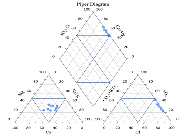
Fig.12: The Piper plot for samples in the study area
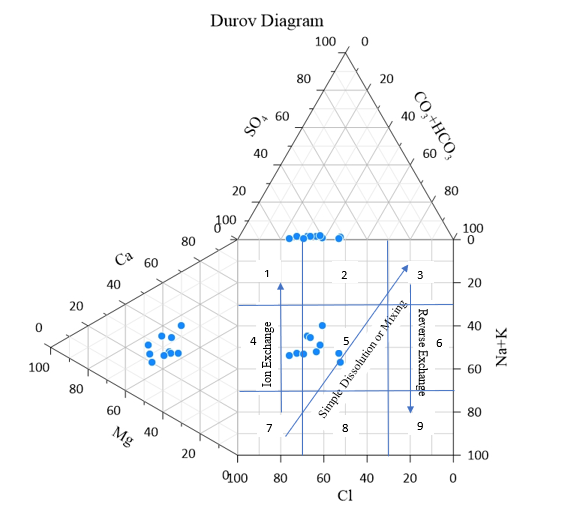
Fig. 13: Durov plot of the acquired hydrochemical data
CONCLUSION
The geology of the study area was composed of the Ameki Formation overlying the Imo Formation. The lithology was composed of sand, clay, and shale, with Ironstone bed in some area. The sediments were generally poorly to moderately sorted, very positively to positively skewed, and platykurtic to leptokurtic. The trend of observations suggests mixed depositional environments and processes. The depositional environment was nearshore/beach, attributed to tidal waves and turbulent current actions. The presence of littoral processes in the linear discriminate analysis further supports this interpretation, highlighting the influence of waves and currents on sediment transport, deposition, and sorting.
The soil samples exhibit moderately to highly plastic behavior suggesting the potential for compressibility and settlement under loading. However, with appropriate compaction techniques and ground improvement measures such as soil stabilization, these soils may be suitable for supporting various engineering structures. The swelling potential of the soil samples, range from medium to high, highlighting the need for careful consideration of the soil’s response to moisture. The sand samples ranged from well-graded to uniformly graded, except for one gap-graded sample. The results suggest favorable shear strength properties, making the soils potentially suitable for roads and infrastructural development. In addition, the well-graded nature implies good drainage properties, low compressibility,
The physical parameters and the major ions in water were within the guideline values. The pH indicates slightly acidic water with values below the permissible limit for drinking water in both surface water and groundwater. The heavy metals chromium, mercury, cadmium, iron, and lead concentrations exceeded the recommended limits in water sources indicating water contamination/pollution. These heavy metals were of particular concern to public health. The heavy metals were mostly of anthropogenic origin through activities such as industrial discharges, municipal waste, and agricultural runoff. Regular monitoring of water quality and implementing appropriate measures, such as effective wastewater treatment systems, improved agricultural practices, and disposal of hazardous waste, are necessary to safeguard human and environmental health. Finally, the dominant hydrochemical facies in the water sources were the Ca2++Mg2+ and Cl– + SO42- with Ca2+ – Mg2+ – Cl– – SO42- as the dominant water type. Additionally, simple dissolution or mixing and ion exchange were the dominant hydrochemical processes that influenced the water chemistry.
REFERENCE
- Adegoke, O. S., Arua, I., and Oyegoke, O. (1980). Two new nautiloids from Imo Shale (Paleocene) and Ameki Formation (Middle Eocene), Anambra State, Nigeria. Journal of Mining and Geology, 17, 85 – 89.
- Allen, G. P. and Posamentier, H. W. (1993). Sequence Stratigraphy and Facies Model of an Incised Valley Fill: The Gironde Estuary, France. Journal of Sedimentary Petrology, 63(3), 378-391.
- Anizoba, D. C, Orakwe, L. C and Chukwuma, E. C. (2020). Assessment of Groundwater Potential of Imo Formation (Ebenebe Sandstone) in Anambra State, Nigeria Using Geo-electrical Sounding Data. Journal of Engineering and Applied Sciences, 16(1), 43-51.
- Anyanwu, N. P. C. and Arua, I. (1990). Ichnofossils from the Imo Formation and their palaeoenvironmental significance. Journal of Mining and Geology 26, 1–4.
- Arua, I. (1980). Palaeocene Macrofossils from the Imo Shale in Anambra State, Nigeria. Journal of Mining and Geology, 17, 81–84.
- Back W, Hanshaw BB. Chemical geohydrology. In: Chow VT (Editor) advances in hydroscience. Academic press. New York. 1965;49-109.
- BSI (1990) BS 1377: 1990—Methods of Test for Soils for Civil Engineering Purposes. British Standards Institute, Milton Keynes.
- Durov SA. Natural waters and graphic representation of their composition. Doklady Akademii Nauk SSSR. 1948;59: 87-90.
- Egboka, B.C., and Okpoko, E.I. (1984). Gully erosion in the Agulu-Nanka region of Anambra State, Nigeria. IAHS-AISH publication, 335-347.
- Ejikeme, J. O., Ojiako, J. C., Onwuzuligbo, C. U., and Ezeh, F. C. (2017). Enhancing food security in Anambra state, Nigeria using remote sensing data. Environmental Review, 6(1), 27-44.
- Folk, R. L. and Ward, W. C. (1957). Brazos River bar: A study in the significance of grain-size parameters. Journal of Sedimentology and Petrology, 27, 3-26.
- Folk, R.L. and Ward, W.C. (1957) A Study in the Significance of Grain-Size Parameters. Journal of Sedimentary Petrology, 27, 3-26.
- Freeze, R.A and Cherry, J.A. (1979). Groundwater. Prentice-Hall, Inc, England Cliffs, N.J.
- Ifeka, A. and Akinbobola, A. (2015). Land use/land cover detection in some selected stations in Anambra State. Journal of Geography and Regional Planning, 8 (1), 1-11.
- Lloyd JA, Heathcote JA. Natural inorganic hydrochemistry in relation to groundwater. An introduction. 1985;296. New York: Oxford Uni. Press.
- Madu, F.M, Okoyeh, E.I, Okolo, C.M, Aseh, P, Elomba, U.F. (2022). Irrigation water quality assessment and hydrochemical facie of Oguta Lake, Southeastern Nigeria. European Journal of Environment and Earth Sciences, 3(1):1– 6.
- Madu, F.M, Okoyeh, E.I, Okolo, C.M, Chibuzor, S.N, Boma, K, Onyebum, T.E and Okpara, A (2022). Physicochemical and Microbial Assessment of Oguta Lake, Southeastern Nigeria. International Journal of Innovative Science and Research Technology, 7 (11), Pg. 2051-2061.
- Mitra, S., Chakraborty, A.J., Tareq, A.M., Emran, T.B., Nainu, F., Khusro, A., Idris, A.M., Khandaker, M.U., Osman, Alhumaydhi, F.A, Simal-Gandara, J. (2022). Impact of heavy metals on the environment and human health: Novel therapeutic insights to counter the toxicity. Journal of King Saud University – Science, 34 (3), 1-21.
- Murthy, V. N. S. (2003). Geotechnical Engineering: Principles and practices of soil mechanics and foundation Engineering. Marcel Dekker, New York.
- Nfor, B. N., Olobaniyi, S. B., & Ogala, J. E. (2007). Extent and distribution of groundwater resources in parts of Anambra state, Southeastern Nigeria. Journal of Applied Sciences and Environmental Management, 11(2), 215–221.
- Ngwoke, K. G., Uzoabaka,T. C., Ezemokwe, I., and Esimone, C. (2015). Levels of Lead and Arsenic in Groundwater and Blood of Residents of Agulu, Nigeria. Polish Journal of Environmental Studies, 24(4), 1717-1721. https://doi.org/10.15244/pjoes/32505
- Nichols, G. (2009). Sedimentology and stratigraphy (2nd ed.). Wiley-Blackwell.
- Nigerian Standard for Drinking Water Quality (NSDQW). (2015). Nigerian Standard for Drinking Water Quality. Nigerian Industrial Standard NIS 554, Standard Organization of Nigeria, pp: 30.
- Nnadi, O., Liwenga, E., Lyimo, J., and Madukwe, M. (2019). Impacts of variability and change in rainfall on gender of farmers in Anambra, Southeast Nigeria. Heliyon, 5(7), 5-12. https://doi.org/10.1016/j.heliyon.2019.e02085.
- Nwajide, C.S. (2013) Geology of Nigeria’s Sedimentary Basins. CSS Bookshop Ltd., Lagos, 1-565.
- Nwajide, C.S., (1980). Eocene tidal sedimentation in the Anambra Basin, Southern Nigeria. Sedimentary Geology 25, 189-207.
- Okolo, C.M., Akudinobi, B.E.B, Obiadi, I.I, Onuigbo, E.N, Obasi, P.N. (2018). Hydrochemical evaluation of lower Niger drainage area, southern Nigeria. Applied water science, 8:201-209
- Okolo, C.M., Akudinobi, B.E.B, Obiadi, I.I. (2020). Evaluation of water resources of some satellite towns in the central part of Anambra State, Se, Nigeria. Sustainable Water Resources Management. 6(6): 102-112.
- Okolo, C.M., Okonkwo, S.O., Madu, F.M, Ifeanyichukwu, K.A. (2024). Assessment of Groundwater Quality around Amaenyi and State Secretariat Dumpsites in Awka, Southeastern Nigeria. Asian Journal of Geographical Research, 7(1), 118-140.
- Onwuemesi, A., Egboka, B., Orajaka, I., & Emenike, E. (1990). Implications of hydrogeophysical investigations of the Agulu-Nanka gullies area of Anambra state of Nigeria. Journal of African Earth Sciences (and the Middle East), 13(3-4), 519-526. https://doi.org/10.1016/0899-5362(91)90114-E.
- Petters, S. W. (1991). Regional Geology of Africa (Lecture Notes in Earth Sciences). Springer-Verlag, Berlin 40, 722-729.
- Piper, A. (1948). A graphic procedure in the geochemical interpretation of water analyses. Am Geophys Union Trans, 25:914–23.
- Posamentier, H. W. and Allen, G. P. (1999) Siliciclastic Sequence Stratigraphy: Concepts and Applications. Vol. 7, SEPM (Society for Sedimentary Geology), Tulsa.
https://doi.org/10.2110/csp.99.07. - Posamentier, H.W. and Allen, G.P. (1999) Siliciclastic Sequence Stratigraphy: Concepts and Applications. Vol. 7, SEPM (Society for Sedimentary Geology), Tulsa.
- Reyment, R. A. (1965). Aspects of the Geology of Nigeria: The stratigraphy of the Cretaceous and Cenozoic deposits, Ibadan University Press, Ibadan, 145.
- Sahu, B. K (1964). Depositional mechanism from the sieve analysis of clastic sediments. Journal of Sedimentary Petrology, 34(1), 73-83.
- Short, K. C., and Stäuble, A. J. (1967). Outline of geology of Niger Delta. American Association of Petroleum Geologists Bulletin 51, 761-779.
- WHO (2011) Guidelines for Drinking Water Quality. 4th Edition World Health Organization, Geneva, Switzerland. http://apps.who.int/iris/bitstream/10665/44584/1/9789241548151_eng.pdf
- Omonona, O.V., and Okogbue, C.O. (2016). Geochemistry of rare earth metals in groundwater of different aquifers in Gboko area, central Benue Trough, Nigeria. Environmental earth science, 76(18); https://doi.org/10.1007/s12665-016-6329-3
- Tolera, M.B., Choi, H., Chang, S.U., and Chung, I.M. (2019). Groundwater quality evaluation for different uses in the lower Ketar Watershed, Ethiopia. Environ Geochem Health.
- Wali, S.U., Alias, N., Harun, S.B. (2020). Hydrogeochemical evaluation and mechanisms controlling groundwater in different geologic environments, Western Sokoto Basin, Northwestern Nigeria. Applied sciences, 2(1808)
- Niyazi, B.A.M., Rajmohan, N., Masoud, M.H.Z., Algarawy, A.M., Elfeki, A., and Rashed, M. (2023). Hydrochemistry and its relationship with groundwater flow and geology in Al Madinah Al Munawarah Province, Kingdom of Saudi Arabia. Journal of Hydrology: Regional Studies.47; https://doi.org/10.1016/j.ejrh.2023.101437.