
Forecasting Performance of Asymmetric GARCH in Stock Market Volatility Models: Relative Potency of EGARCH and PGARCH Models
- Godwin Chigozie Okpara
- Nzeadibe Okechukwu Henry
- 663-674
- Mar 22, 2025
- Economics
Forecasting Performance of Asymmetric GARCH in Stock Market Volatility Models: Relative Potency of EGARCH and PGARCH Models
Godwin Chigozie Okpara.1, Nzeadibe Okechukwu Henry2
1Department of Banking and Finance, Abia State University Uturu
2Department Economics, College of Education Arochukwu
DOI: https://doi.org/10.51584/IJRIAS.2025.10020056
Received: 26 January 2025; Accepted: 31 January 2025; Published: 22 March 2025
ASYMMETRIC VOLATILITY
Asymmetric volatility phenomenon is a market dynamic which shows that there are higher market volatility levels in market downswings (negative shocks) than in market upswings (positive shocks). It implies that volatility tends to increase in response to bad news and decrease in response to good news (Okpara, 2016). In other words, the presence of asymmetric volatility is mostly apparent during stock market crisis when a large decline in stock price is associated with a significant increase in market volatility (Wu 2001). This implies that negative surprises have a much greater effect on volatility than do positive ones. This situation is commonly associated with the financial market where ‘bad news’ (negative shocks) is found to have larger impact on volatility than good news (positive shocks) of the same magnitude.
Researchers such as Christie (1982), Schwert (1989) and Nelson (1991) observe that when bad news reaches the stock market, future volatility generally increases while good news of the same magnitude does not cause sharp increase in future volatility. In other words, a sharp price drop increases the stock return volatility but a price rise of the same magnitude leads to lower volatility of stock return. Asymmetric volatility is linked to financial leverage.
Black (1976) first found the asymmetric volatility and attributed it to changes in financial leverage. Christie (1982) in her work also attributed asymmetric volatility to effects stemming from changes in financial leverage (debt-equity ratio). The leverage effect theory maintains that a decrease in the price of stock (bad news) will lead to an increase in financial leverage (debt to equity ratio) implying that firms will be highly geared. Asymmetric effects where negative shocks (bad news) cause the value of the firms to fall will have the effect of raising the debt-equity ratio which is synonymous with the increase in the risk of bankruptcy. This will make the stock riskier and increase the volatility of returns. Although to many, “leverage effects” have become synonymous as asymmetric volatility, the asymmetric nature of the volatility response to return shocks could simply reflect the existence of time-varying risk premiums (Pindyck, 1984, French, Schwert and Stambaugh, 1987 and Campbell and Hentschel, 1992). The measured effect of stock price changes on volatility is too large to be explained solely by financial leverage changes. The leverage effect explains why a lower return leads to a higher volatility; while the volatility feedback effect shows how higher volatility may reinforce a lower return. The volatility feedback theory states that an increase in expected volatility will lead to a decrease in stock demand due to risk aversion.
Review of Relevant Asymmetric Models
Asymmetric models used for this analysis are the exponential GARCH models, the threshold GARCH model and the Power GARCH model. We shall explain each of these model as follows.
EGARCH in Mean Model
The GARCH model developed by Bollerslev (1986) imposed limitations that impair the capturing of positive or negative sign of the error term ut as to determine the impact of negative and positive shocks on conditional volatility. To him, both signs of shocks have the same impact on conditional variance. The GARCH model though reckoned for its simplicity unarguably is not without shortcomings. For instance, fitting the model becomes difficult when it involves more than one lag on each of the explanatory variables. Secondly, it negates the effects of shock on its signs where as in actuality evidence of asymmetric response abound in the financial market especially in the stock market. In the GARCH model, only the squared residual enters the conditional variance equation thereby rendering the signs of the residuals no effect on conditional volatility. The GARCH (p,q) model for conditional volatility is written as follows.
\(\sigma_1^2 = \omega_0 + \sum_{i=1}^{p} \alpha_i \epsilon_{t-i}^2 + \sum_{j=1}^{q} \beta_j \sigma_{t-j}^2\),
where \(\alpha_i > 0\) and \(\beta_j > 0\) are conditions for the conditional variance, \(\sigma_t^2\), to be always positive.
While \(\sum_{i=1}^{q} a_i + \sum_{j=1}^{p} \beta_j < 1\) is the condition for stationarity.
Thus, the case of the GARCH model depends on three terms, namely, the mean \(\omega_0\), news on volatility of the last period \(\epsilon_{t-i}^2\), which is the ARCH term, and the last period’s forecast variance known as the GARCH term.
If the conditional variance is introduced into the mean equation, the ARCH in mean (ARCH-M) model is derived:
\(Y_t = X_t^1 Y_t + Y_2 \sigma_{t-1}^2 + \epsilon_t\)
This is often used in financial applications where the expected return on an asset is related to the expected asset risk. However, it is often the case that the conditional variance, \(\sigma_t^2\), is not an even function of the past disturbances, \(U_{t-1}, U_{t-2}, \dots, U_{t-n}\), an important feature often observed when analyzing stock market returns (Koulakiotis, Papasyriopoulos, and Molyneux, 2006).
To address this feature, Nelson (1990) proposed the exponential GARCH model, which incorporates leverage effects and observed asymmetric volatility changes with changes in return signs. In his model, the log of conditional variance implies that the leverage effect is exponential rather than quadratic and that forecasts of the conditional variance are guaranteed to be nonnegative.
In other words, the exponential GARCH model is a refinement of the GARCH model, as it allows conditional variance to respond asymmetrically to return innovations of different signs. Nelson (1991) proposed this model (EGARCH) to allow for asymmetric effects between positive and negative asset returns. The EGARCH model adopts the device of making the natural logarithm of the variance, \(\ln\sigma^2\), linear in some functions of time and lagged error terms. In other words, it is formulated in terms of the logarithm of conditional variance. The model for conditional variance is specified as follows:
\(\ln\sigma_t^2 = \omega + \beta\ln\sigma_{t-1}^2 + \alpha \left[ \frac{|\epsilon_{t-1}|}{\sigma_{t-1}} – \frac{2}{\pi} \right] + \gamma \frac{\epsilon_{t-1}}{\sigma_{t-1}}\)
Where:
- \(\omega, \beta, \alpha, \gamma\) are constant parameters,
- \(\ln\sigma_t^2\) = the one-period-ahead volatility forecast,
- \(\omega\) = the mean level,
- \(\beta\) = persistence parameter,
- \(\alpha\) = volatility clustering coefficient,
- \(\ln\sigma_{t-1}^2\) = the past period variance,
- \(\gamma\) = the leverage effect.
Unlike the GARCH model, the EGARCH model allows for a leverage effect.
In the analysis of the relationship between expected returns and expected volatility, the augmented version of the EGARCH-in-mean model is usually employed in order to capture the leverage effect. The choice of the method stems from the fact that in a developing economy for instance, the market consists of risk-averse investors as the opportunity to invest and diversify the investment is not much. Thus, the expected returns on asset should significantly move in the same direction with the expected risk of the asset. We therefore state the return equation as follows
\(R_t = b_0 + b_1 R_{t-1} + b_2 \sigma_t^2 + \epsilon_t \quad \ldots 20.12\)
Where:
- \(R_t = \text{stock market returns at time } t\)
- \(R_{t-1} = \text{last period return accounting for autocorrelation}\)
- \(\sigma_t^2 = \text{the conditional variance}\)
- \(b_2 \sigma_t^2 = \text{market rise premium for expected volatility}\)
- \(\epsilon_t = \text{the usual idiosyncratic term with zero mean and conditional variance } \sigma_t^2.\)
This expected volatility, which is approximated by the conditional variance \(\sigma_t^2\), is related to the information set up such that:
\[
\sigma_t^2 = \operatorname{var}(R_t \mid \psi_{t-1})
\]
Where:
- \(\psi_{t-1}\) is the information set at time \(t-1\) containing observations on lagged values of \(R_t\) and \(\sigma_t\). That is, \(\sigma_{t-1}, \sigma_{t-2}, \ldots, R_{t-1}, R_{t-2}, \ldots\)
Thus, the expected returns on an asset should significantly move in the same direction as the expected risk of the asset. In light of this, one can state the return equation together with the log of the conditional variance equation as follows in 20.13 and 20.14. These equations were jointly estimated:
\[
R_t = b_0 + b_1 R_{t-1} + b_2 \sigma_t^2 + \epsilon_t \quad \ldots 20.13
\]
\[
f_{R-1}, f_{\delta_t^2} > 0
\]
\[
\epsilon_t / \psi_{t-1} \sim N(0, \sigma_t^2)
\]
\[
\epsilon_t = z_t \sigma_t \text{ and } z_t \sim N(0, 1)
\]
\[
\ln \sigma_t^2 = \omega + \beta \ln \sigma_{t-1}^2 + \alpha \left[ \frac{|\epsilon_{t-1}|}{\sigma_{t-1}} – \sqrt{\frac{2}{\pi}} \right] + \gamma \frac{\epsilon_{t-1}}{\sigma_{t-1}} \quad \ldots 20.14
\]
\[
f_{\delta_t^2} > 0, \quad f_\alpha, \quad f_\gamma < 0
\]
The parameters have been previously defined
The conditional variance \(b_2\) and the persistent parameter are expected to be positive, while the volatility clustering coefficient and the leverage effect coefficients should be negative. If the estimated variance can be used to predict expected returns in equation 20.6, then the value of \(b_2\) should be positive and significant for a risk-averse investor. That is to say that the higher the risk of an investment, the higher the reward accruable for having undertaken such a risky investment.
The EGARCH-M model, a refinement of the GARCH model, imposes a non-negativity constraint on market variance and allows for conditional variance to respond asymmetrically to return innovations for different signs. If \(\gamma\) is negative, that is \(\gamma < 0\), leverage effect exists. If \(\gamma \neq 0\), then the impact is asymmetric. Black (1976) was the first to note that changes in stock returns display a tendency to be negatively correlated with changes in returns volatility. The leverage effect phenomenon posits that volatility tends to rise in response to “bad news” and to fall in response to “good news.” That is, an unexpected drop in price (bad news) increases predictable volatility more than an unexpected increase in price (good news) of similar magnitude (Black, 1976; Christe, 1982).
In other words, a negative value of \(\gamma\) indicates that volatility is higher when returns are negative. \(\gamma\) is called the “sign effect.” If \(\alpha\) is positive, then the conditional volatility tends to rise (fall) when the absolute value of the standardized residuals is larger (smaller). \(\alpha\) is called the “magnitude effect.”
Threshold-GARCH
Another extension of the classic GARCH model, called Threshold-GARCH, that allows for the leverage effect was proposed by Jean-Michel Zakoian (1990). The Threshold-ARCH (TARCH) model divides the distribution of the innovations into disjoint intervals and then approximates a piecewise linear function for the conditional standard deviation. Rabemananjara and Zakoian (1993), by including the lagged conditional standard deviations as a regressor, extended the preliminary model to be known as Threshold GARCH (TGARCH). TGARCH is estimated with the following equation:
\[
\sigma_t^2 = a_0 + \sum_{i=1}^{p} a_i \epsilon_{t-i}^2 + \sum_{i=1}^{p} \gamma_i S_{t-i} \epsilon_{t-i}^2 + \sum_{j=1}^{q} b_j \sigma_{t-j}^2
\]
Where:
\[
S_{t-i} = \begin{cases}
1 & \text{if } \epsilon_{t-i} < 0 \\
0 & \text{if } \epsilon_{t-i} \ge 0
\end{cases}
\]
The effects of \(\epsilon_{t-i}\) on the conditional variance \(\sigma_t^2\) will depend on whether the error term \(\epsilon_{t-i}\) is above or below the threshold value, which is always zero. The squared error \(\epsilon_{t-i}^2\) will have different effects on the conditional variance \(\sigma_t^2\) as follows:
- If \(\epsilon_{t-i}\) is positive, total effects are given by \(\epsilon_{t-i}^2\).
- If \(\epsilon_{t-i}\) is negative, total effects are given by \((a_i + \gamma_i) \epsilon_{t-i}^2.\)
In the case of the TGARCH method, \(\gamma\) represents the asymmetric effect, and it is expected to be positive and significant for bad news to have a greater effect on volatility than good news, implying that the leverage effect exists. The \(\gamma\) coefficient is negative, that is \(\gamma < 0\), if there is no leverage effect.
PGARCH Model
The model is given as follows:
\[
\sigma_t^d = a_0 + \sum_{i=1}^{p} a_i (|\epsilon_{t-i}| + \gamma_i \epsilon_{t-i})^d + \sum_{j=1}^{q} b_j \sigma_{t-j}^d, \quad d > 0, \; |\gamma_i| \le 1 \; \forall \; i = 1,2,\ldots,r
\]
Where:
- \(\sigma_t^d\) = Estimated conditional variance at time \(t\)
- \(a_i\) and \(b_j\) = Residual and variance coefficients, respectively
- \(\epsilon_{t-i}\) = Residual from previous periods
- \(\sigma_{t-j}^d\) = Lagged variance from period \(t-j\)
- \(d\) = Positive coefficient representing the value of the power term
The GARCH term \(b_j\) estimates the volatility clustering of the conditional variance. If the GARCH term is significant, it indicates that volatility is clustered, meaning periods of high volatility and low volatility are observed.
The parameter \(\gamma\) represents the leverage effect, which captures the asymmetric feature of volatility. When \(d = 2\) and \(\gamma = 0\), the equation reduces to the classic GARCH model. For the model to capture asymmetric effects, \(\gamma\) must not be zero, meaning \(\gamma \neq 0\).
When \(d = 1\), the conditional standard deviation is estimated. The flexibility of the PGARCH model can be increased by treating \(d\) as another coefficient to be estimated, as suggested by Zivot (2008).
MATERIALS AND METHODS
In discussing GARCH models, the researcher bears in mind of two categories of GARCH and choose the one appropriate to his investigation. The two categories are the symmetric models which are made up of GARCH (1,1) and GARCH-M (1,1) models, the next is the Asymmetric models which are made up of the Exponential GARCH (EGARCH 1,1) model, the Power GARCH (PGARCH 1,1), Threshold GARCH (TGARCH 1,1), Glosten, Jagannathan and Runkle (GJRGARCH) model, Quadratic GARCH (QGARCH) and others in the family of asymmetric GARCH models. In all this study, we shall apply the EGARCH and PGARCH models not only to estimate the conditional hetroscedasticity of the models but also to test for the more efficient model using the diagnostic ARCH-LM test of coefficients of the models as well as the Akaike and Schewatz information criteria.
Data employed for these analysis are the daily all share index (ASI) of the Nigerian Stock Exchange (NSE) from 1st February 2001 to 11th August 2018 resulting in 4423 observations excluding public holidays. The daily all share index (ASI) series are used to generate the continuously compounding returns used in the Asymmetric GARCH modeling. The compounding returns are given as follows:
100*ln(P_t/P_(t-1) ) = 100[ln(P_(t ))-ln〖(P〗_(t-1))]
Where R_t represents the continuously compounded daily percentage returns of the ASI for period t and t-1. P_t and P_(t-1 ) represent current and past daily prices. For lack of space, the data are not provided in this work but may be made available on request. In this analysis, the researcher first of all looked at the descriptive statistics of the NSE’s continuously compounding daily return series over the period 1/2/2001 to 11/8/2018 to observe the behavior of the sourced data in terms of mean, median, standard deviation, skewness, kurtosis, Jarque Bera and others.
Table 4.1 Descriptive Statistics for Stock Returns
| RT | |
| Mean | -0.031054 |
| Median | 0.000246 |
| Maximum | 11.04592 |
| Minimum | -11.40446 |
| Std. Dev. | 1.028414 |
| Skewness | -0.118686 |
| Kurtosis | 11.95810 |
| Jarque-Bera | 14795.98 |
| Probability | 0.000000 |
| Sum | -137.3207 |
| Sum Sq. Dev. | 4675.810 |
| Observations | 4422 |
Table 4.1 showing the descriptive statistics of the return series indicates that the series ranges from minimum of -11.40446 to maximum of 11.04592 with a mean value of -0.031054. The Jarque-Bera is 14795.98 with a probability value of 0.000000 which is significant at the 1% level thereby indicating that the distributed population of the return series are not normal. The skewness is negative (-0.118686) suggesting that the distribution of the variable has a long left tail. The kurtosis of 11.95810 is greater than the usual kurtosis of 3 implying that the distribution is leptokurtic. Thus, the observed skewness and kurtosis also show that the distribution of daily stock return series is non normal.
The trend line snapshot view for the daily returns for examining the stationarity of the data suggests that the data are stationary. The daily return series graph is presented in fig.4.1 as follows.
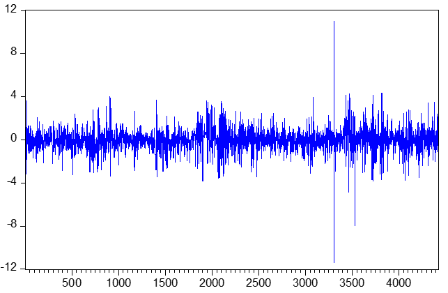
Fig.4.1 Graph of the Daily Return series
The graph suggests that the data on returns are stationary at the level. To authenticate this using the Augmented Dickey-Fuller unit root test (Dickey and Fuller, 1979), the unit root test is checked by fitting a regression on equation based on a random walk with an intercept drift term \((\vartheta)\) as follows.
\[
\Delta y_t = \vartheta + \delta y_{t-1 } + \sum \phi_j y_{t-1} + \mu_t
\]
Where \(\mu_t\) is a stochastic term. The null hypothesis here is:
\[
H_0: \delta=0 \quad \text{against the alternative hypothesis} \quad H_1; \delta<0.
\]
If the value of ADF test statistics exceeds the value of Mackinnon critical value, the null hypothesis is rejected and there is no unit root in the series. The unit root test is presented at the level \(n\) table 4.2 as follows.
Table 4.2 Unit root Test at the level.
| Null Hypothesis: RT has a unit root | ||||
| Exogenous: Constant | ||||
| Lag Length: 0 (Automatic – based on SIC, maxlag=30) | ||||
| t-Statistic | Prob.* | |||
| Augmented Dickey-Fuller test statistic | -41.94291 | 0.0000 | ||
| Test critical values: | 1% level | -3.431646 | ||
| 5% level | -2.861998 | |||
| 10% level | -2.567057 | |||
| *MacKinnon (1996) one-sided p-values. | ||||
From table 4.2, we can see that the Augmented Dickey Fuller test statistic is -41.94291 which is more negative than the critical value at 1% level (which is -3.431646). This confirms that the return series are stationary at the level. Thus, the graphical assertion has been authenticated.
Asymmetric Models Analysis
Based on the forgoing, the researcher focused on exponential generalized autoregressive conditional hetroscedasticity in mean (EGARCH in Mean) model and Power generalized autoregressive conditional hetroscedasticity (PARCH) Model analyses. The two models using Akaike and Schewarz information criteria are compared in order to determine the one that is better fitted to the model. We however ran the model first using the least squared method and checked the residuals of this model. the least square method of the model is presented in table 4.3.
Table 4.3 Least Square Method
| Dependent Variable: RT | ||||
| Method: Least Squares | ||||
| Date: 03/01/20 Time: 15:31 | ||||
| Sample (adjusted): 3 4423 | ||||
| Included observations: 4421 after adjustments | ||||
| Variable | Coefficient | Std. Error | t-Statistic | Prob. |
| RT1 | 0.430563 | 0.013576 | 31.71388 | 0.0000 |
| C | -0.017542 | 0.013968 | -1.255861 | 0.2092 |
| R-squared | 0.185403 | Mean dependent var | -0.030880 | |
| Adjusted R-squared | 0.185219 | S.D. dependent var | 1.028465 | |
| S.E. of regression | 0.928347 | Akaike info criterion | 2.689629 | |
| Sum squared resid | 3808.415 | Schwarz criterion | 2.692522 | |
| Log likelihood | -5943.425 | Hannan-Quinn criter. | 2.690649 | |
| F-statistic | 1005.770 | Durbin-Watson stat | 1.994550 | |
| Prob(F-statistic) | 0.000000 | |||
From the OLS model, we check the residuals. It should be noted that the existence of hetroscedasticity is a precondition for applying the GARCH models to a financial time series data and as such provides justification for volatility modeling using the GARCH models. The result of the residuals is presented in fig.4.4 as follows.

Fig 4.2 Residuals of the Model
Fig 4.2 showing the residual plot elucidates that there are long periods with low fluctuations as well as long periods with high fluctuations implying that periods of low volatility tends to be followed by periods of low volatility for a prolonged period and periods of high volatility is followed by periods of high volatility for a relatively short period. Such consistent behavior of residuals suggests the use of ARCH family models. To authenticate this fact, we ran a hetroscedasticity test. The result of the hetroscedasticity test is presented in table 4.4 as follows.
Table 4.4 Hetroscedasticity test.
| Heteroskedasticity Test: ARCH | ||||
| F-statistic | 905.3762 | Prob. F(1,4418) | 0.0000 | |
| Obs*R-squared | 751.7340 | Prob. Chi-Square(1) | 0.0000 | |
The result of the hetroscedaticity test in table 4.4 shows that the probability value of F and the observed R2, all are less than 5% indicating the presence of ARCH effect. We further confirm this using the correlogram and Ljung-Box Q- statistics test for Hetroscedasticity.
Table 4.5 Correlogram and Ljung-Box Q- statistics Test for Hetroscedasticity.
| Date: 03/08/20 Time: 06:37 | ||||||
| Sample: 2 4423 | ||||||
| Included observations: 4422 | ||||||
| Autocorrelation | Partial Correlation | AC | PAC | Q-Stat | Prob | |
| |*** | | |*** | | 1 | 0.431 | 0.431 | 820.28 | 0.000 |
| |* | | | | | 2 | 0.180 | -0.006 | 963.97 | 0.000 |
| | | | | | | 3 | 0.030 | -0.055 | 968.09 | 0.000 |
| | | | | | | 4 | 0.001 | 0.010 | 968.09 | 0.000 |
| | | | | | | 5 | -0.009 | -0.004 | 968.42 | 0.000 |
| | | | | | | 6 | -0.035 | -0.037 | 973.84 | 0.000 |
| | | | | | | 7 | -0.022 | 0.008 | 975.95 | 0.000 |
| | | | | | | 8 | -0.011 | 0.002 | 976.52 | 0.000 |
| | | | | | | 9 | 0.028 | 0.038 | 980.02 | 0.000 |
| | | | | | | 10 | 0.028 | 0.002 | 983.47 | 0.000 |
| | | | | | | 11 | 0.017 | -0.003 | 984.77 | 0.000 |
| | | | | | | 12 | 0.018 | 0.013 | 986.20 | 0.000 |
| | | | | | | 13 | 0.016 | 0.005 | 987.30 | 0.000 |
| | | | | | | 14 | 0.022 | 0.013 | 989.36 | 0.000 |
| | | | | | | 15 | 0.012 | -0.001 | 989.99 | 0.000 |
| | | | | | | 16 | 0.016 | 0.013 | 991.15 | 0.000 |
| | | | | | | 17 | 0.004 | -0.007 | 991.23 | 0.000 |
| | | | | | | 18 | 0.018 | 0.021 | 992.70 | 0.000 |
| | | | | | | 19 | 0.022 | 0.009 | 994.77 | 0.000 |
| | | | | | | 20 | 0.013 | -0.003 | 995.54 | 0.000 |
| | | | | | | 21 | 0.038 | 0.039 | 1001.8 | 0.000 |
| | | | | | | 22 | 0.063 | 0.042 | 1019.3 | 0.000 |
| | | | | | | 23 | 0.029 | -0.025 | 1023.1 | 0.000 |
| | | | | | | 24 | 0.037 | 0.033 | 1029.3 | 0.000 |
| | | | | | | 25 | 0.018 | -0.006 | 1030.7 | 0.000 |
| | | | | | | 26 | 0.045 | 0.043 | 1039.7 | 0.000 |
| | | | | | | 27 | 0.068 | 0.045 | 1060.6 | 0.000 |
| | | | | | | 28 | 0.056 | 0.006 | 1074.4 | 0.000 |
| | | | | | | 29 | 0.017 | -0.019 | 1075.7 | 0.000 |
| | | | | | | 30 | -0.008 | -0.010 | 1076.0 | 0.000 |
| | | | | | | 31 | 0.004 | 0.015 | 1076.1 | 0.000 |
| | | | | | | 32 | -0.006 | -0.012 | 1076.2 | 0.000 |
| | | | | | | 33 | -0.018 | -0.015 | 1077.6 | 0.000 |
| | | | | | | 34 | -0.017 | -0.001 | 1079.0 | 0.000 |
| | | | | | | 35 | -0.010 | -0.002 | 1079.4 | 0.000 |
| | | | | | | 36 | 0.003 | 0.002 | 1079.4 | 0.000 |
Using Ljung-Box Q-statistics to check for validity of autoregressive conditional hetroscedaticity (ARCH) in the residuals, it is found that since the values of autocorrelations and partial autocorrelations are not zero at all lags and since the Q statistics are significant, there is clear evidence that the return series exhibits ARCH effects. In other words, if there is ARCH in the residuals, the autocorrelations and partial autocorrelations should not be zero at all lags and the Q statistics should be significant. Thus, by this decision rule, we conclude that there exists ARCH effects in the return series. The conclusion therefore informs the use of GARCH models which are designed to deal with time series hetroscedasticity. The researcher therefore confidently compare the efficiency of EGARCH-in Mean and PGARCH methodology in working on the time series hetroscedasticity. The EGARCH in Mean model is presented in table 4.6 as follows.
Table 4.6 EARGARCH in Mean Model
| Dependent Variable: RETURNS | ||||
| Method: ML ARCH – Normal distribution (BFGS / Marquardt steps) | ||||
| Sample: 2001 4479 | ||||
| Included observations: 2479 | ||||
| Convergence achieved after 25 iterations | ||||
| Coefficient covariance computed using outer product of gradients | ||||
| Presample variance: backcast (parameter = 0.7) | ||||
| LOG(GARCH) = C(4) + C(5)*ABS(RESID(-1)/@SQRT(GARCH(-1))) + C(6) | ||||
| *RESID(-1)/@SQRT(GARCH(-1)) + C(7)*LOG(GARCH(-1)) | ||||
| Variable | Coefficient | Std. Error | z-Statistic | Prob. |
| GARCH | -0.019880 | 0.038946 | -0.510450 | 0.6097 |
| RT1 | 0.495144 | 0.016208 | 30.54907 | 0.0000 |
| C | 0.040870 | 0.024215 | 1.687835 | 0.0914 |
| Variance Equation | ||||
| C(4) | -0.316298 | 0.023358 | -13.54131 | 0.0000 |
| C(5) | 0.340646 | 0.027633 | 12.32755 | 0.0000 |
| C(6) | -0.032595 | 0.012995 | 2.508207 | 0.0121 |
| C(7) | 0.903765 | 0.010408 | 86.83494 | 0.0000 |
| R-squared | 0.345491 | Mean dependent var | 0.046702 | |
| Adjusted R-squared | 0.344962 | S.D. dependent var | 1.013347 | |
| S.E. of regression | 0.820146 | Akaike info criterion | 2.283149 | |
| Sum squared resid | 1665.456 | Schwarz criterion | 2.303570 | |
| Log likelihood | -2827.921 | Hannan-Quinn criter. | 2.293113 | |
| Durbin-Watson stat | 1.663530 | |||
Table 4.7 ARCH LM TEST
| Heteroskedasticity Test: ARCH | |||
| F-statistic | 0.376997 | Prob. F(1,2476) | 0.5393 |
| Obs*R-squared | 0.377244 | Prob. Chi-Square(1) | 0.5391 |
The coefficients estimated for the stock return as presented in table 4.7 shows that there are no more ARCH effects as the F statistic is not significant at 5 percent critical level. Thus, we conclude that there are no more ARCH effect in the residual using EGARCH in mean model. This therefore justifies the efficiency of EGARCH-in-mean model in estimating the conditional volatility of the stock returns. The GARCH parameter representing the conditional variance is negative, suggesting that the stock exchange in Nigeria is a negative and insignificant function of conditional variance. The researcher, at this point estimates the PARCH model to examine the performance so as to compare the models. The result of the PARCH model estimation is presented in table 4.8 as follows:
Table 4.8 The result of the PGARCH Model
| Dependent Variable: RETURNS | ||||
| Method: ML ARCH – Normal distribution (BFGS / Marquardt steps) | ||||
| Sample: 2001 4479 | ||||
| Included observations: 2479 | ||||
| Convergence achieved after 49 iterations | ||||
| Coefficient covariance computed using outer product of gradients | ||||
| Presample variance: backcast (parameter = 0.7) | ||||
| @SQRT(GARCH)^C(8) = C(4) + C(5)*(ABS(RESID(-1)) – C(6)*RESID( | ||||
| -1))^C(8) + C(7)*@SQRT(GARCH(-1))^C(8) | ||||
| Variable | Coefficient | Std. Error | z-Statistic | Prob. |
| GARCH | -0.002055 | 0.039197 | -0.052419 | 0.9582 |
| RT1 | 0.497374 | 0.016459 | 30.21910 | 0.0000 |
| C | 0.027921 | 0.024757 | 1.127783 | 0.2594 |
| Variance Equation | ||||
| C(4) | 0.066919 | 0.008331 | 8.032285 | 0.0000 |
| C(5) | 0.192466 | 0.017661 | 10.89762 | 0.0000 |
| C(6) | -0.085751 | 0.042609 | -2.012508 | 0.0442 |
| C(7) | 0.752683 | 0.019595 | 38.41100 | 0.0000 |
| C(8) | 1.353554 | 0.217721 | 6.216928 | 0.0000 |
| R-squared | 0.345918 | Mean dependent var | 0.046702 | |
| Adjusted R-squared | 0.345389 | S.D. dependent var | 1.013347 | |
| S.E. of regression | 0.819879 | Akaike info criterion | 2.285759 | |
| Sum squared resid | 1664.370 | Schwarz criterion | 2.304526 | |
| Log likelihood | -2825.198 | Hannan-Quinn criter. | 2.292575 | |
| Durbin-Watson stat | 1.668914 | |||
Table 4.8 confirms that the conditional variance is negatively and insignificantly related to the stock market in Nigera. In other words, the stock market is a negative and insignificant function of conditional volatility in Nigeria.
Table 4.9 Heteroskedasticity Test: ARCH
| F-statistic | 0.213069 | Prob. F(1,2476) | 0.6444 |
| Obs*R-squared | 0.213223 | Prob. Chi-Square(1) | 0.6443 |
The persistent parameter β(C5) is positive and significant indicating (or confirming) the existence of clustering feature in the volatility of the stock market in Nigeria. The asymmetric coefficients are negative and significant implying that there is asymmetric effect and leverage effect in the Nigerian stock market. The Power term estimate as presented in table 4.8 is 1.353554. In the light of this, the researcher resort to diagnostic test by applying ARCH LM test on the residuals to check whether PGARCH model is efficient enough in explaining conditional heteroskedasticity of the stock returns. The Heteroskedasticity test is presented in table 4.9
The result from table 4.9 shows that there are no longer ARCH effects in the model.
The persistent parameter is positive and significant indicating that the stock market volatility is persistent.
Comparing the Schwarz Information Criteria of the two models, it is seen that while the Schwarz Information Criteria for the EGARCH in mean Model is 2.303570, the Schwarz Information Criteria for PARCH model is 2.304526. Thus, Science the Schwarz information criteria in EGARCH in mean Model is less than that of PARCH model, the EGARCH in mean model is robust and more efficient for estimation Asymmetric Models
CONCLUSION
In the mean equation, the GARCH parameters which is the stock market conditional volatility exerts a negative and insignificant impact on the stock market. In other words, the stock market return is a negative and insignificant function of conditional volatility.
The persistent parameter β is positive and significant confirming the existence of clustering features in the volatility of the stock market in Nigeria.
The asymmetric coefficients are negative and significant implying that there is asymmetric effect and leverage effect in the Nigerian stock market suggesting that unexpected drop in price (bad news) increases predictable volatility more than an expected increase in price \(good news) of similar magnitude in the country.
Comparing the efficacy of the two models, it is found that the EGARCH in mean Model is more efficacious or so to say much more Robust and efficient than the PARCH Model in estimating the asymmetric GARCH Models since the values of both Akaike Information Criteria and the Skewatz Information Criteria are lower in EGARCH in Mean than in PARCH Model.
REFERENCES
- Black, F. (1976), “Stock of stock price volatility changes”, in proceedings of the 1976 meetings of the business and Economic statistics section.
- Bollerslev, T. (1986) “Generalized autoregressive conditional heteroskedasticity”, Journal of econometricians,. 31:30-327.
- Christie, A.A. (1982} The stochastic behavior of common stock variances. Journal of financial economics 10, 407-432
- Engle, R.F. (1982) “Autoregressive conditional heterscedasticity with estimates of the variance of an United Kingdom inflation”, Econometrica, 50:987-1008.
- Koulakiotis, A., Papasyriopoulos, N. and Molyneux, P. (2006) “More evidence on the relationship between stock price returns and volatility”, Journal of finance and economics.
- Leon, N.K. (2008) Stock market returns and volatility in the BRVM. African journal of business management, 15, 107-112, August.
- Nelson, D. (1991) ‘Conditional heteroskedastcity in asset returns: a new approach’, Econometrica,. 45: 347-370
- Christie, A.A. (1982) The Stochastic Behaviour of Common Stock Variances: Value, Leverage and Interest Rate Effects. Journal of Financial Economics, 10, 407-432 .
- Schwert, G. W. (1989). Why does market volatility change over time? Journal of Finance, 44(5), 1115-1153..
- Nelson, D.B. (1991) Conditional Heteroskedasticity in Asset Returns A New Approach. Econometrica Journal of the Econometric Society, 59, 347-370.
- R Pindyck ·( 1984) Risk, Inflation, and the Stock Market. Robert Pindyck · American Economic Review, 1984,. 74, issue 3, 335-51.
- K French, Kenneth French, G. Schwert and Robert Stambaugh (1987) Expected stock returns and volatility, Journal of Financial Economics, 19, issue 1, 3-29..
- Campbell, J.Y. and Hentschel, L. (1992) No News Is Good News: An Asymmetric Model of Changing Volatility in Stock Returns. Journal of Financial Economics, 31.
- Koulakiotis, A., Papasyriopoulos, N., P. Molyneux (2006) More evidence on the relationship between stock price returns and volatility: A note, Journal of Finance.
- Daniel B. Nelson (1990)Stationarity and Persistence in the GARCH(1,1) Model.Econometric Theory, 6, issue 3, 318-334.
- Nelson, D.B. (1991) Conditional Heteroskedasticity in Asset Returns A New Approach. Econometrica Journal of the Econometric Society, 59, 347-370.
- R Rabemananjara and Jean-Michel Zakoian ( 1993) Threshold Arch Models and Asymmetries in Volatility. Journal of Applied Econometrics, 8, issue 1, 31-49.
- Dickey, D.A.I. and Fuller, W.A. (1979) Distribution of the Estimators for Autoregressive Time Series with a Unit Root. Journal of the American Statistical Association, 74, 427-431..
- Zivot, E. (2008): Predicting Stock Volatility Using After-Hours Information. Unpublished manuscript, Department of Economics, University of Washington.
- Lawrence R Glosten, Ravi Jagannathan and David E Runkle(1993) Journal of Finance, 48, issue 5, 1779-1801.
- Kenneth French, G. Schwert and Robert Stambaugh (1987)Expected stock returns and volatility, Journal of Financial Economics, 19, issue 1, 3-29.
- John Campbell and Ludger Hentschel (1992)An asymmetric model of changing volatility in stock returns. Journal of Financial Economics, 31, issue 3, 281-293.
- Wu, H. (2001) Fractions (Draft), http://www. math.berkeley.edu/~wu/. 5.
- Pindyck, Robert S ( 1984), “Risk, Inflation, and the Stock Market.” The American Economic Review, 74, Issue. 3, 335-51