Submission Deadline-26th July 2024

July 2024 Issue : Publication Fee: 30$ USD Submit Now

Submission Open

Special Issue of Education: Publication Fee: 30$ USD Submit Now

Model Validation for an Integrated Solar PV System Laboratory

Aminu Alhaji Abdulhamid
Jibrin Abdullahi
194-222
May 8, 2024
Micronutrient

Model Validation for an Integrated Solar PV System Laboratory

Aminu Alhaji Abdulhamid, Jibrin Abdullahi

Department of Electrical and Electronic Engineering Technology, Isa Mustapha Agwai I Polytechnic, Lafia

DOI: https://doi.org/10.51584/IJRIAS.2024.904014

Received: 08 February 2024; Revised: 24 February 2024; Accepted: 29 February 2024; Published: 08 May 2024

ABSTRACT

This study focuses on the model validation of an Integrated Solar System Laboratory, employing a comprehensive approach encompassing solar energy sources, batteries, DC/DC boost converters, inverters, and controllers. Mathematical models were meticulously formulated for each key component and implemented using MATLAB/Simulink to create a virtual environment mirroring the laboratory setup. Validation was conducted by accurately representing the designed system parameters in the simulation environment, and then assessing the dynamic responses of the various simulated outputs. The system, designed for diverse photovoltaic solar applications, integrates energy management software. Simulation results showcase the system’s dynamic responses to varying solar irradiance, load patterns, and disturbances, highlighting the efficacy of control algorithms. Key findings indicate that the incremental conductance algorithm effectively optimizes the PV module’s operating point at 7.5 Amps and 90 volts. System stability endures load variations, with the inverter stable at 65%. Additionally, the efficiency of the MPPT technique and converter duty cycle stability are emphasized, along with the battery discharge rate reduction from 67% to approximately 20%. The study validates solar system models, ensuring accurate representation. Robust control algorithms maintain stability amidst load variations, showcasing system efficiency.Keywords: Model validation, Integrated Solar System Laboratory, Energy management software, solar irradiance, Control algorithms.

INTRODUCTION

The global demand for renewable energy sources has intensified as nations strive to address environmental concerns, energy security, and sustainable development. In the context of Nigeria, a nation endowed with abundant solar resources, harnessing solar energy presents a viable pathway towards meeting the country’s increasing energy needs while minimizing its carbon footprint [1]. However, despite the significant potential of solar energy, there exists a substantial gap between theoretical knowledge and practical skills within the Nigerian solar energy industry [2].

The solar energy sector in Nigeria is poised for substantial growth, driven by government initiatives, international commitments to reduce carbon emissions, and the need for decentralized energy solutions [3]. However, the effective integration of solar technologies into the energy landscape requires a skilled workforce equipped with hands-on experience and a profound understanding of cutting-edge technologies such as smart grid systems, Internet of Things (IoT) connectivity, energy management software, and hybrid renewable systems [4]. Recognizing this imperative, this study introduced an innovative educational initiative – an automated modular solar energy training laboratory specifically tailored to address the unique challenges and opportunities within the Nigerian context. The innovative laboratory aims to go beyond conventional theoretical teaching methodologies, incorporating state-of-the-art technologies and industry-aligned curriculum to empower students with practical skills essential for the evolving landscape of the solar energy sector.

This study contributes vital insights to the field of renewable energy by offering a comprehensive understanding of the dynamic interactions within solar power systems. The optimized control strategies and enhanced efficiency of energy harvesting will pave the way for more reliable and scalable renewable energy solutions. Findings from this study will guide future developments in renewable energy systems, facilitating their integration into mainstream energy grids and promoting sustainability.

Aims and Objectives

This study aims to perform model validation for the Integrated Solar System Laboratory, ensuring that the developed models accurately reflect the dynamic behavior of the integrated solar system components. The specific objectives were to formulate precise mathematical models for key components within the integrated solar system, including solar energy sources, batteries, DC/DC boost converters, inverters, and controllers; utilize MATLAB/Simulink to implement the mathematical models, creating a virtual environment that faithfully reproduces the laboratory’s integrated solar system; and, conduct extensive validation through comparison of the simulated outputs with real-world data from the Integrated Solar System Laboratory to ensure the accuracy and reliability of the developed models.

System Architecture

The developed automated solar energy training laboratory is a compact and modular prototype designed for comprehensive student learning, with dimensions not exceeding 2.0 meters in length, 1.7 meters in height, and 0.4 meters in depth. It has a sturdy construction, a modern appearance, and integrated workstations. Solar panels on top generate electricity, while displays provide real-time system data. The prototype combines functionality and aesthetics, efficiently utilizing space for training at Isa Mustapha Agwai I Polytechnic, Lafia Nigeria. The system architecture is shown in Figure 1.

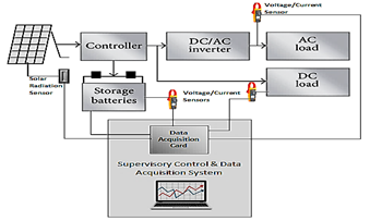
Figure 1: Block Diagram of the System

System Description

The system shown in Figure 1 comprises a solar energy source, battery storage, DC/DC boost converters with MPPT control, an inverter with a controller, and loads. This system is designed to replicate various photovoltaic solar applications, aiming to deliver stable and reliable power. Modeling and control are crucial for operational analysis. The simulation model includes a solar energy source, energy storage, MPPT control, and associated conditioning units. A PWM inverter controller regulates three-phase AC bus voltage and frequency. A DC-DC buck/boost converter control strategy maintains constant DC link voltage during power source or load changes. The system is implemented for effective laboratory instruction at Isa Mustapha Agwai I Polytechnic (IMAP), Lafia, as well as various scenarios across Nigeria.

The system also features a workstation with a display for monitoring and managing solar systems. It integrates smart grid simulation, IoT connectivity, and energy management software. Hybrid renewable systems and energy-efficient technologies are included. The console empowers students to gain practical experience and contribute to solar energy education.

RELATED LITERATURE

Existing literature presents compelling evidence for the modeling and validation of integrated solar power systems, showcasing diverse approaches and applications. A transient model for a solar hybrid pilot plant was successfully validated by [7] in Spain, demonstrating accurate integration of photovoltaic-thermal collectors, thermal storage, and a reversible heat pump. The system’s self-sufficiency in meeting varied energy demands highlights the model’s robustness. In another study, [6] explored optical-thermal and classical thermal models for a solar PV system, addressing varying and constant coefficients with incident angle variations. Their comprehensive approach, involving astronomical calculations and electromagnetic theory, resulted in accurate predictions validated against experimental data. The significant agreement between the classical thermal model and actual electricity production attests to its modeling accuracy and reliability. Furthermore, [5] validated detailed photovoltaic (PV) models for building-integrated systems, emphasizing the importance of addressing partial shading and thermal impacts. Their optical-thermal-electrical model, incorporating a five-parameter PV cells circuit, accurately predicted power production under shading conditions. The model’s ability to improve accuracy during severe mismatching and accurately predict temperatures underscores its value in assessing integrated PV systems’ effects on power losses and hot spots. A thorough modeling and validation of a solar PV plant was conducted by [8] using field-measured data. The study aimed to authenticate model accuracy, covering both steady-state and dynamic models. An algorithm fine-tuned gains for electrical and plant controllers, confirming its efficacy in capturing dynamic intricacies during a capacitor bank switching event.

Together, these studies and many others contribute valuable insights into the modeling and validation of integrated solar power systems, offering approaches applicable to different contexts, such as hybrid pilot plants, general PV systems, and building-integrated systems. These findings collectively emphasize the importance of accurate modeling techniques in optimizing the performance and reliability of solar energy systems across diverse applications and conditions.

METHODOLOGY

Detailed mathematical models were developed for key components, including the solar photovoltaic system, battery storage/management system, DC/DC boost converters, and inverter. Utilizing relevant equations and fundamental physics principles, these models were used to accurately portray the behavior of each component in the system. MATLAB/Simulink simulation tools played a central role in converting the formulated mathematical models into a virtual environment. This involved creating a comprehensive simulation setting that incorporated the solar energy source, energy storage, MPPT control, and conditioning units. A robust control strategy was developed for the DC/DC boost converters and the inverter, prioritizing power flow optimization, voltage and frequency regulation, and overall system stability. In addition, MPPT control algorithms were implemented to improve the efficiency of energy harvesting from the solar source.

A. Matlab Implementation: Simulink-Simscape Modeling

The Matlab model implementation initiates with the creation of a single-line representation of the system using Simulink-Simscape. The methodology, adopted in this study, employs Simulink-Simscape, a block diagram modeling language in Matlab tailored for multi-domain physical systems.

Parameterization Process: To set system parameters, components are configured by double-clicking and inputting model and control values into designated fields within the parameter block. This parameterization step involves providing predetermined model parameters for each selected system component from the advanced Simulink-Simscape library.

Automatic Scripting: Matlab then automatically converts these configured parameters into code, generating M-code, C-code, or PLC-Code as required. This seamless transition from the Simulink-Simscape environment to executable code ensures the accurate representation and implementation of the designed model.

1. Photovoltaic System Modelling

The Current-voltage (I -V) characteristics of a typical PV module are shown in Figure 3. The current axis (where V = 0) is the short-circuit current I_SC, and the intersection with the voltage axis (where I = 0) is the open-circuit voltage V_OC. The power as a function of voltage is also shown in Figure 2. The locus of maximum power points is also shown. The maximum power that can be obtained corresponds to the rectangle of maximum area under the I–V curve. At the maximum power point the power is P_mp, the current is I_mp, and the voltage is V_mp. Ideally, cells would always operate at the maximum power point, but practically cells operate at a point on the I-V curve that matches the I-V characteristic of the load. Current-voltage (I-V) curves are shown in Figure 3 for the selected PV module (Sun Power SPR-E20-327) operating at a fixed temperature and at several irradiation levels. For the module, short-circuit current increases in proportion to the solar radiation, while open-circuit voltage increases logarithmically with solar radiation. As long as the curved portion of the I-V characteristic does not intersect the current axis (where V = 0), the short-circuit current is nearly proportional to the incident radiation.

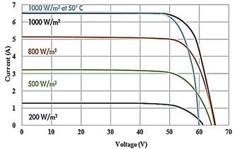
Figure 3: The I-V Curves for the selected PV module (Sun Power SPR-E 20-327) at Several Irradiation Levels.

The single-diode model was employed owing to its suitability for system design purposes. This model requires several parameters that are characteristic of the cell/s being modeled. The parameters are not directly given in the manufacturers’ datasheets for commercial PV modules. They need to be extracted from the datasheet information. Figure 4 is an equivalent circuit that can be used for an individual cell, a module consisting of several cells, or an array consisting of several modules. As seen from the Figure, the light-intensity dependent current source I_ph is connected in parallel with a forward biased diode I_D, while the two parasitic resistances R_sh and R_S modeling the module losses are connected as shown in Figure 4.

Figure 4: Equivalent Circuit for the PV System Model

At a fixed temperature and solar radiation, the external (load) current of this model is given as expressed by [12] as:

I=I_ph-I_D-I_sh (1)

Where;

I = Load Current

I_ph=The Photon Current

I_D=Diode current=I₀ (e^{(q(V+IR_s)/akT)}-1)

I_{(Rsh )}=Shunt Resistance Current=(V+IR_S)/R_sh

Thus;

I=I_ph-I_o [e^{(q(V+IR_s)/akT)}-1]-(V+IR_s)/R_sh (2)

Where;

I_ph=Photon Current

R_sh=Shunt Resistance

R_S=Series Resistance

I₀=Reverse (dark)Saturation Current

a=Diode Ideality Factor

For most practical applications, there are multiple PV cells connected in series to form a PV module (as shown in Figure 5), which in turn are arranged to form PV arrays. It therefore means that the equivalent model for the circuit in Figure 5 can be represented as;

I=I_ph-I_o [e^{q(V+IRS )/(N_sakT)}-1]-(V+IR_s)/R_sh (3)

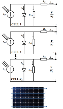
Figure 5: Arrangement of Series-Connected PV Cells

As stated earlier, the datasheets do not directly give the five parameters needed for modeling the PV cell. They however provide enough data to derive these parameters. Hence using the datasheet information on open circuit voltage (Voc), short circuit current (Isc), maximum power point voltage (Vmp), maximum power point current (Imp), temperature at STC, Irradiance at STC, number of series-connected cells for the module and indeed maximum power at STC; we can extract the five parameters using equation (3). As stated earlier, these are:

Photon Current (I_ph ),

Shunt Resistance (R_sh ),

Series Resistance (R_S ),

Reverse (dark)Saturation Current(I₀ ); and

a=Diode Ideality Factor.

The Photon Current (I_ph): At short circuit conditions and under standard test conditions (STC), the external (or) load voltage is zero (V = 0), therefore; I = I_SC = I_ph, since the voltage drops across the shunt and series resistances are very small (and therefore negligible).

Thus;

I_SC=I_ph (4)

So that to obtain the photon current at any given operating condition, we scale it suitably using the expression;

I_ph=(I_{SC_STC}+K₁ ∆T) G/G_STC (5)

Where; G = Solar irradiance in W⁄m² at any given operating condition;

G_STC=Solar irradiance in W⁄m² at STC;

I_{SC_STC}=Short circuit current at STC from datasheets;

K₁=Temperature Coefficient of I_{SC_STC};

∆T=Temperature difference between

cell temperature and its temperature at STC (25˚C).

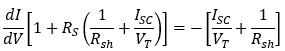
The Shunt Resistance (R_sh): Under short circuit conditions, the shunt resistance affects the slope of the I-V curve inversely. Therefore, differentiating equation (3) we have;

dI/dV=I₀/V_T [e^{(V+IR_S)/V_T )} (1+R_S∙dI/dV)]-1/R_sh -R_S/R_sh ∙dI/dV

(Note that: The Thermal Voltage (V_T )=akT/q, so that q/akt=1/V_T )

Then;

dI/dV [1+R_S/R_sh+(I₀R_S)/V_Te^{(V+IR_S)/V_T)}] = I₀/V_T ∙e^{((V+IR_S)/V_T )}– 1/R_sh (6)

Therefore under any given operating condition we have;

dI/dV=(I₀/V_T ∙e^(V+IRS)/VT)-1/R_sh )/(1+R_s/R_sh +(I_oR_s)/V_T ∙e^{(V+IR_s)/V_T )} (7)

But we are concerned specifically with short circuit conditions under which the reverse saturation current I₀=0, and R_S has typically very small values, and hence R_S≪R_sh. Thus;

dI/dV=-1/R_sh

So that at short circuit conditions;

R_sh=-dV/dI (8)

The Series Resistance (R_S): The series resistance significantly impacts on the slope of the I-V curve near the open circuit conditions. Under these conditions, no external current flows in the system, and the only current present is the reverse (dark) saturation current (I₀). Thus, under open circuit conditions;

More importantly,

I_SC-V_OC/R_sh ≈I_SC-0≈I_SC

This is because under open circuit conditions, R_sh≫V_OC. Hence equation (6) becomes;

On rearranging, we have;

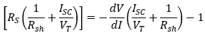
So that;

(9)

But at open circuit conditions,

1/R_sh ≪I_SC/V_T

Since R_shis usually very large; hence:

R_S=dV/dI-V_T/I_SC (10)

Where

V_T=(N_S akT)/q

(Note that with the exception of the diode ideality factor ‘a’, all other terms in the expression are either known constants or readily available from datasheets of the selected PV module).

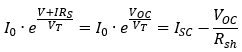
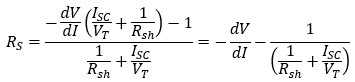
Reverse (Dark) Saturation Current (I₀): Under open circuit conditions, the terminal voltage (V) is the open circuit voltage (V_OC) with its value at the maximum, while the short circuit current (I_SC) approaches and eventually becomes zero. Thus; V=V_OC, I=0 & I_SC=I_ph. Equation (3) then becomes;

(11)

But

e^{(V_OC/V_T )}≫1;

Therefore:

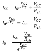(12)

Diode Ideality Factor (a): The diode ideality factor is a measure of the material quality. This means that lower values reflect better diode material, lower reverse saturation and higher power output. Its impact is predominantly near the maximum power point on the I-V curve; and this can be used to estimate the value of ‘a’ from datasheets of the given PV module. The values of ‘a’ range from 1 to 2. At maximum power point conditions; V=V_mp & I=I_mp. So that equation (3) becomes;

I_mp=I_SC-I₀ [e^{(V_d/V_T )}-1]-V_d/R_sh

Where; V_d=V_mp+R_S I_mp

Thus;

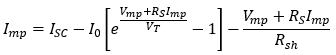(13)

So that ‘a’ can be obtained from the expression;

V_T=(N_S akT)/q

Equations (10), (12) and (13) were parameterized in the Simulink model blocks with respect to the parameters ‘R_S’, ‘I₀’ and ‘a’. The selected PV module is SunPower SPR-E20-327; a 327W (peak power) monocrystalline flat plate, and its datasheet information is as given in Table 1. Two additional details which are not given explicitly in the datasheets are: the slope of the I-V curve near the short circuit conditions, and; the slope of the I-V curve near the open circuit conditions. These can however be estimated from the I-V curves shown in Figure 3.

Table 1: Datasheet information for SunPower SPR-E20-327 Monocrystalline Solar PV Module

Parameter	Symbol	Value
Nominal Power (+5/-0%)		327 W
Cell Efficiency	η	22.5%
Panel Efficiency	η	20.4 %
Rated Voltage		54.7 V
Rated Current		5.98 A
Open-Circuit Voltage		64.9 V
Short-Circuit Current		6.46 A
Maximum System Voltage (as per IEC)		600V UL; 1000 IEC
Temperature Coefficients	Power (P)	– 0.38%/°C
	Voltage (V_OC)	– 176.6mV/°C
	Current (I_SC)	3.5mA/°C
Number of Cells in Series		96
NOCT		45°C +/– 2°C
Series Fuse Rating		20A
Limiting Reverse Current (3 strings)		16.2A
Grounding		Positive Grounding not required

The PV system modeled using Simscape as shown in Figure 6, implements up to 11 series-connected PV panels arranged in an array of 8 parallel strings, making a total of 88 connected PV panels to give a net power of 28.776kW.

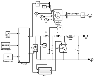
Figure 6: Simulink Model for the PV System

The values along with other defined parameters are used in the Simulink Model blocks to configure the model characteristics into a real-time PV system, which can be tailored to fit varying scenarios based on user pre-defined inputs on the system workstation.

2. Modeling of the Battery Energy Storage System

The lead-acid battery model is determined by equation (14), which depending on the state of function vary between + or -, the first one is for the charging state and the second one is for the discharging state as is described in [14].

V=E_m±IR (14)

Where V is the terminal voltage, I, is the actual current used by an external charge (which in idle state is approximated to 0) and 𝑅 is the internal resistance, which vary depending on different parameters such as capacity, charge/discharge current, temperature, among others, and E_m is the open circuit voltage defined by equation (15):

E_m=E_m0-K_e(273+T_e)(1-SOC) (15)

From equation (15), E_m0 is the open circuit voltage at maximum charge, K_e is a constant granted by datasheet, T_e is the electrolyte temperature and 𝑆𝑂𝐶 is the state of charge, which can be found applying equation (16).

SOC=(q-q_dis)/q_max (16)

Where 𝑞 is the actual battery charge calculated by the result of I×t, q_dis is the actual battery discharge rate and q_max is the battery capacity. The size of battery storage is important, and detailed calculations should be made to meet the demand when the power from the electric grid is not available. [15] suggested that the required battery capacity is given as:

B_size=(E_load×Days_off)/(DoD_max×η_temp ) (17)

Where

Eload =the load that needs to be supplied during unavailability of power in ampere hour

Daysoff =the storage days (the days that power from the electric grid is unavailable)

DoDmax =the maximum depth of discharge of the battery

ηtemp =the temperature correction factor

According to [13], the charge quantity of the storage system is given by:

E_B (t)=E_B (t-1)∙(1-ζ)+(E_GA (t)-(E_L (t))/η_inv )∙η_Batt (18)

Where ζ_ηinv and η_batt are the hourly self-discharge factor, efficiency of inverter, and efficiency of the battery, respectively; E_B (t) and E_B (t-1) are the charge quantity of storage system at time t and t-1, correspondingly; and E_GA and E_L are the renewable energy power and load demand, respectively. The charge quantity is constrained by maximum and minimum charge quantities E_Bmax and E_Bmin, respectively [7].

Due to the varying nature of the internal resistance (for different battery types), many battery system models have been proposed based on the experimental identification of the battery parameters; such as TRNSYS model proposed by [12], Kinetic Battery Model reported by [16], etc. Hence the kinetic battery model, simple in approach, is more commonly employed for multiple DER applications. The Kinetic Battery model is a two-tank model with kinetics that best describes lead acid battery behavior [17]; [18]. The first tank contains “available energy,” or energy that is readily available for conversion to DC electricity. The second tank contains “bound energy,” or energy that is chemically bound and therefore not immediately available for withdrawal. Three parameters are used to describe this two tank system. Eckstein further pointed out that the maximum (or theoretical) storage capacity (Qmax) is the total amount of energy the two tanks can contain. The total amount of energy stored in the Storage Component at any time is the sum of the available and bound energy, hence:

Q=Q₁+Q₂; (19)

Where Q1 is the available energy and Q2 is the bound energy.

[18] suggested that the maximum amount of power that the storage can absorb over a specific length of time is given by the equation:

P_batt,dma,kbm=(-kcQ_max+kQ₁e^-k∆t+Qkc(1-e^-k∆t ))/(1-e^-k∆t+c(k∆t-1+e^-k∆t ) ) (20)

where:
	Q1	= the available energy [kWh] in the storage at the beginning of the time step
	Q	= the total amount of energy [kWh] in the storage at the beginning of the time step
	c	= the storage capacity ratio [unitless]
	k	= the storage rate constant [h-1]
	Δt	= the length of the time step [h]

Similarly, the maximum amount of power that the Storage Component can discharge over a specific length of time (Δt) is given by the following equation:

P_batt,dma,kbm=(kQ₁ e^-k∆t+Qkc(1-e^-k∆t))/(1-e^-k∆t+c(k∆t-1+e^-k∆t ) ) (21)

On calculating the actual charge or discharge power, the resulting amount of available and bound energy at the end of the time step is calculated using equations (22) and (23):

Q_1,end=Q₁ e^-k∆t+((Qkc-P)(1-e^-k∆t )/k)+(PC(k∆t-1+e^-k∆t )/k) (22)

Q_2,end=Q₁ e^-k∆t+Q(1-c)(1-e^-k∆t)+(P(1-C)(k∆t-1+e^-k∆t)/k) (23)

where

Q1 = the available energy [kWh] at the beginning of the time step

Q2 = the bound energy [kWh] at the beginning of the time step

Q1,end = the available energy [kWh] at the end of the time step

Q2,end = the bound energy [kWh] at the end of the time step,

P = the power [kW] into (positive) or out of (negative) the storage bank

Δt = the length of the time step [h]

Figure 6 shows the implemented the battery energy storage system model in Simulink. It implements the battery charging limits, the reactive power capability and the total storage capacity.

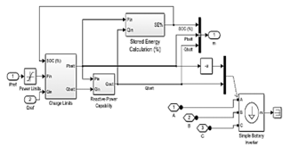
Figure 7: Model for the Energy Storage System (ESS)

The charging limits were dictated by the round trip efficiency (as designed earlier); the reactive power capability depending on the control signals from the load, as well as the dispatch from the PV system; while the storage capacity is parameterized as earlier designed. The ESS model also implements the system converter and system controller models exactly as they are implemented in the PV system model.

3. Modeling of the Charge Controller

The employed MPPT controller adopted the incremental conductance method, chosen for its efficiency in tracking maximum power under rapidly changing atmospheric conditions. This technique adjusts the PV module terminal voltage based on incremental and instantaneous conductance, aligning it with the Maximum Power Point (MPP) voltage. The correlation between dI/dV and -I/V signifies the controller’s ability to identify MPP location. The instantaneous conductance (-I/V) value of the system and incremental conductance (dI/dV) values are useful in determining the maximum power point on the P-V curve. The algorithm uses the information of source voltage and current to find the desired operating point. The equations according to [9] were used to implement Simulink model of MPPT using the incremental conductance technique as follows:

dI/dV=-I/V at MPP (24)

dI/dV>-I/V left of MPP (25)

dI/dV<-I/V right of MPP (26)

Using equations (24), (25) and (26), the algorithm shown in Figure 8 was used to select the most suitable step-sizes for various adjustments corresponding to the solar irradiation at each instance.

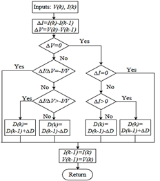
Figure 8: MPPT Algorithm for the Implemented Incremental Conductance

The PWM control signal of the converter is regulated by the MPPT until the condition (dI/dV+I/V=0) occurs, and in order to maintain a continuous power flow between the DC terminal and battery storage device with constant DC link voltage, a buck/boost DC-DC converter is used; with 2 PI control loops to regulate the DC-link voltage as shown in Figure 9. The reference DC link voltage of 144V is considered, so that the DC bus voltage will remain stable during changes in either the source power or load variations.

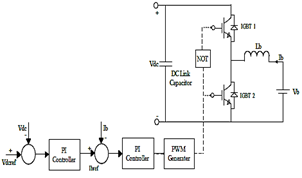
Figure 9: IC-MPPT-Driven Control Strategy for the Buck-Boost converter

The inner loop of the control system effectively manages battery current, providing resilience against parameter variations. Simultaneously, the outer loop maintains control of the voltage regulation. To uphold power balance amidst fluctuating source power and dynamic load conditions, the battery undergoes controlled charging or discharging processes. As illustrated in Figure 9, the two IGBTs in the converter operate in a complementary fashion, driven by the PWM signal. The voltage V_dc is then compared with a reference voltage (V_dcref) to derive an error signal. Subsequently, I_bref is compared with the battery current to generate a PWM signal. The obtained error is compensated by the PI controller, as shown.

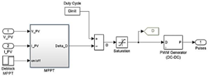
Figure 10: Simulink model of the MPPT Charge Controller

The implemented Simulink model shown in Figure 10 incorporates an MPPT controller based on the incremental conductance method. Simulink Library components are utilized based on the algorithm; employing equations (24), (25), and (26) from [9]. To determine adjustment steps for the PV module terminal voltage, the algorithm dynamically selects suitable step-sizes for adjustments corresponding to changes in solar irradiation at each instance. Signal Processing blocks are used to calculate incremental conductance (dI/dV) and instantaneous conductance (-I/V), and thus; identify the Maximum Power Point (MPP) on the P-V curve. The model then integrates the correlation between dI/dV and -I/V to locate the MPP on the curve. The parameterized PWM block in the model regulates the control signal of the converter based on the MPPT algorithm. A buck/boost DC-DC converter ensures continuous power flow between the PV system and the battery storage device. Two Proportional-Integral (PI) control loops are integrated into the model to regulate the DC-link voltage, thereby maintaining stability. The model considers a reference DC link voltage of 144V. This reference voltage ensures the stability of the DC bus voltage even during changes in source power or load variations.

4. Modeling of the Inverter

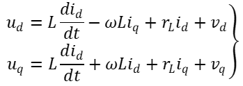
The system inverter was designed by initiating control of the output voltage and frequency based on the state-space average models of a single-phase half-bridge inverter in real and imaginary stationary reference frames as obtained by [10].

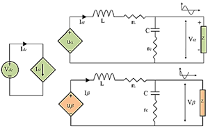
Figure 11: Stationary Reference Frames Model of Single-Phase Inverter [10]

From the circuit model shown in Figure 11,

(27)

(28)

Where;

V_dc=constant voltage source

U_α=dependent ‘real’ voltage source

U_β=dependent ‘virtual’ voltage source

I_α=dependent current source

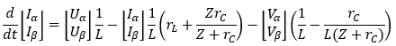
After obtaining the average real and imaginary models, as expressed in equations (27) and (28), the d-q model of the inverter can be derived by applying the transformation matrix equations (29) and (30) to these averages. Hence;

(29)

(30)

Where T is the transformation matrix; and:

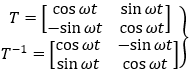(31)

This results in:

(32)

(33)

By applying the chain rule to equations (32) and (33), and separating the ‘d’ and ‘q’ components; the state space model can be obtained as follows:

(34)

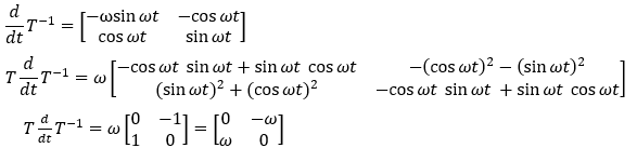
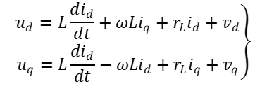
(35)

Equations (35) and (34) (also known as the d-q equations) can be simplified by neglecting r_L and r_c as in practice, they have negligible values. It is worth noting that the cross coupling terms occur between d and q components in the simplified equations as follows:

(36)

(37)

As seen from equation (36), the inductor cross-coupling is adequately addressed, while equation (37) adequately addresses the capacitor coupling; between the d and q components.

The Simulink implementation of the single-phase, full sine wave inverter is shown in Figure 12. The model was implemented in Simscape by integrating specific library blocks, including PLL & Measurements for grid synchronization, V_dc Generator for modeling the DC link voltage, Current Regulator for inverter current regulation, V_{abc_ref} Generation (max m = 1) for generating reference ABC voltages, and PWM Generator for generating Pulse Width Modulation (PWM) signals.

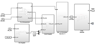
Figure 12: Simulink Implementation of the System Inverter

The PLL & Measurements block was connected to the grid voltage, and its output was linked to the V_dc Generator block. The Current Regulator block received the output of the V_dcGenerator block, regulating the inverter current. The V_{abc_ref} Generation block, configured with ‘max m = 1,’ generated reference values within permissible limits based on the current regulation. The PWM Generator block was connected to the V_{abc_ref} Generation block, generating PWM signals to control the inverter switches.

The PWM Generator block was subsequently linked to the inverter switches and load. Throughout the design process, careful parameter adjustments were made to meet the specific requirements and ratings of a 30kVA inverter system. The completed Simulink model represents the entire control system of the inverter, encompassing grid synchronization; current control, voltage reference generation, and PWM signal generation. Feedback loops and additional control features were incorporated to enhance system stability and performance. Detail of parameterization and math-modeling of each block is reflected under its mask as shown.

5. The Inverter Controller Modeling

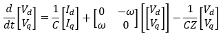
Using the state space approach, the inverter modelling dynamics are defined at medium to high frequencies. The DC-link voltage changes very slowly over the time, owing to the action of the DC-link capacitor. Thus controller structure and the closed-loop model for the inverter would adopt an approach in the synchronous rotating reference frame, so that the continuous-time state equation for the inverter in the d-q coordinate system would depend on our already developed inverter model. Therefore equations (34) and (35) can be re-written as:

(38)

So that the coupling terms in equation (38) derived from equations (34) and (35) can be decoupled in equation (39). Thus;

(39)

Where u_d and u_q are the control signals, v_d and v_q are the inverter output voltage components in the d-q frame respectively. It is possible to derive the controller equations by integrating equation (39), with the adoption of the Backward Euler method over the sampled period (k-1) T_S to kT_S. The di/dt variation is averaged over one sampling period and dividing by T_S. So that;

di_d/dt≈(i_d,k-i_d,k-1)/T_S (40)

di_q/dt≈(i_q,k-iq,k-1)/T_S (41)

Using the Backward Euler method suggested by [11], the output current variation between two consecutive samples i_k and i_{k-1/_{can be approximated to average levels. Thus;}}

i_d,k≈(i_d,k+i_d,k-1)/2 (42)

i_q,k≈(i_q,k+i_q,k-1)/2 (43)

Where i_k and i_k-1 are the d-q reference currents at the sampling instants k and k-1, respectively. This results in:

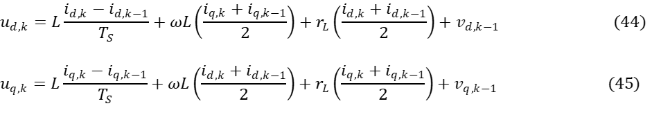
Assuming that the current error is eliminated in one sampling interval, the current at instant k equal the current reference at instant k-1 (i’_d,k-1), then;

i_d,k=i’_d,k-1
i_q,k=i’_q,k-1

The assumption is made that the fundamental output voltage remains constant during a single sampling period, with the sampling frequency typically being several times faster than the highest frequency component in the output voltage. That is:

v_d,k≈v_d,k-1
v_q,k≈v_q,k-1

From the foregoing it is seen that the PI control signal employed within the d-q controller in stand-alone mode is expressed as:

The integral term is computed by multiplying the integral gain with the accumulated sum of recent errors. The steady-state error is represented as the sum of past errors within the integral component of the PI controller. Specifically, the steady-state current error is equivalent to the cumulative sum of previous current errors, leading to:

Where m represents intermediate discrete samples, and the resulting PI-controller is given as:

(48)

where k_p=(L/T_S +r_L/2), k_C=ωL, T_i=(r_L/((L/T_S +r_L/2) )

The closed loop system configuration is shown in Figure 13, while the Simulink implementation is illustrated by Figure 14.

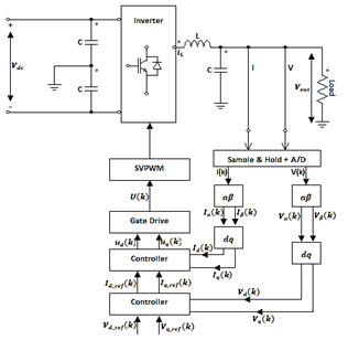
Figure 13: The Controller Closed Loop System Configuration

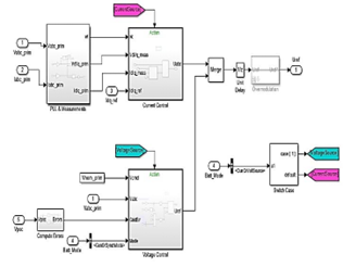
Figure 14: The Inverter Controller Simulink Implementation

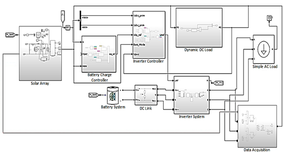
Figure 15: Simulink Model of the Complete System

6. The Complete System

The complete Simulink model of the system, (shown in Figure 15) encompassing the solar array, boost converter, DC/AC inverter, data acquisition block, and control unit, incorporated diverse control algorithms with ideal switches assumed in power converters. Simulink standard blocks implement relevant equations for a comprehensive system model, featuring 11 series-connected PV panels in 8 parallel strings, providing a net power of 28.776 kW. The single-diode model, suitable for system design, necessitates parameter extraction from datasheets. The battery storage system mirrors the PV system, incorporating charging limits, reactive power capability, and total storage capacity. The charge controller adopts an MPPT controller with a buck/boost DC-DC converter ensuring continuous power flow. Two PI control loops regulate DC-link voltage stability. The inverter model, implemented with specific library blocks, ensures control over output voltage and frequency. The synchronous rotating reference frame is adopted for controller stability, encapsulating the entire system for effective analysis and optimization.

The data acquisition block was implemented in Simulink, using signal lines, math blocks, and specific library blocks for data acquisition. Signal lines connected the data block to system points for real-time data monitoring. Simulink library blocks interfaced with sensors, acquired data, and processed signals. Sequencing in the subsystem ensured a logical flow: signals from sensors were routed to the data acquisition block via input ports, capturing information on voltage, current, and temperature. Math blocks facilitated signal conditioning, preparing data for analysis or recording within the Simulink environment, thereby ensuring an efficient, synchronized data flow. The system configuration parameters are presented in Table 2.

Table 2: System Configuration Parameters

Parameter	Value/Unit	Symbol
Total Array Voltage	122.8 Volts	V
Total Array Current	9.8 Amps	A
Total Array Rated Power	28.776 kilo-Watt	kW
Maximum Allowable Load Profile	160 kilo-watt-hour	kWhr
Maximum System Storage Capacity	4.8 kilo-Ampere-hour	kAh
Inverter System Capacity	10kW x 3 Segregated Single-Phase Circuits	kW
System Charge Controller Capacity	100 Amps 12V/24V/48V CDC	A
Battery Initial State of Discharge	70%	–

RESULTS AND DISCUSSION

This section presents simulated system responses under different operating conditions within the Matlab/Simulink environment, employing a simulation time of 3.0 seconds. Utilizing the SunPower SPR-E20-327 Monocrystalline Solar PV Module (see Table 1 for Datasheet Information) and specified simulation parameters (Table 2), the study mirrors real-world conditions by integrating NREL’s daily global solar radiation data for Lafia, Nigeria, focusing on January. The battery controller maintains a constant DC bus voltage, and a PWM inverter controller regulates AC bus voltage and frequency. With the reference DC-link voltage set at 144V and the Lead-Acid battery initialized at a 70% charge, the analysis explores variations in solar irradiation and load conditions through activated resistive and reactive load banks.

I-V and P-V Curves for Selected PV Module, alongside Maximum Power Evaluation in Complete Array:

In Figure 16, the I-V (a) and P-V (b) Curves depict the performance of the selected PV Module, while the Locus of Maximum Power for the Complete Arrays is shown in (c). This figure provides a comprehensive view of the system’s behavior, emphasizing the critical role of incremental conductance algorithm in discerning the optimal operating point for dynamic responses under varying conditions. At the maximum power point, the current (I_mp) is 7.5 Amps, and the voltage (V_mp) is 90 volts. The oscillation of the operating point around the MPP highlights the algorithm’s effective tracking and adjustment to changing conditions.

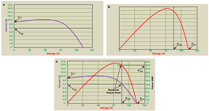
Figure 16: I-V and P-V Curves for the selected PV Module (The Locus of Maximum Power is also shown for the Complete Array (c))

B. Responses of Key System Parameters with Changing Load Patterns

In Figure 17, the dynamic responses of key system parameters under varying disturbances are illustrated. The system initiation at 15.5kW experiences a load increase to 17kW with an additional 5kVars of reactive load at 0.75 seconds. Subsequently, around 1.9 seconds, an extra 3kVars load is introduced. The inverter output initially drops from the optimal 27.8kW to about 20kW, while the system inertia, managed by inverter controller outputs, mitigates the resulting frequency swings to maintain stable voltage and frequency. Remarkably, the combined PV/BESS output remains largely unaffected during these contingencies, affirming the robust stability control algorithms of both the inverter and charge controller.

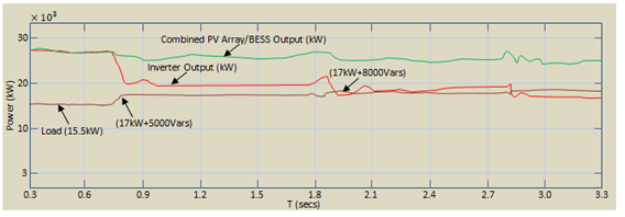
Figure 17: PV Power and Inverter Power at Various Loads

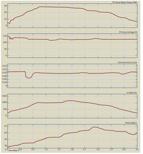
Figure 18: Simulation Result for PV and Converter Outputs at Different Temperature and Irradiance Levels

C. Dynamic Responses of the PV Array, Charge Controller, and System Converter

The simulation graph in Figure 18 depicts the dynamic responses of the PV array, charge controller, and system converter to varying solar irradiance and PV cell temperature. The simulation is scaled at 0.1375 seconds = 60 minutes, representing a single day. The incremental conductance MPPT technique, embedded in the system controller and dedicated converters, optimizes PV array output under different temperature and irradiance conditions. Throughout the simulation, the converter duty cycle remains relatively constant at 0.50, showcasing the system’s efficiency in adapting to environmental changes for enhanced energy harvesting.

D. System Integration/Coordination

In Figure 19, an integrated analysis of system components is presented, evaluating responses to simulated dynamic load changes. From 4 to 5 seconds into the system initiation, the main load switch triggers, causing a 65% drop in cumulative AC load to below 50% and a swing in controllable DC load from 75% to 80% and then below 50%. Notably, the inverter output initially dips from 93%, stabilizing at around 65% to maintain system stability. The battery discharge remains stable at 67% after the initial dip (from 93%) until approximately T = 1 second. Subsequently, the discharge rate eases to nearly 20% as the PV output increases with the rise in solar irradiance. This showcases the robust stability control algorithms of both the system converter and controller as further seen in the fidelity demonstrated by the actual DC link voltage in Figure 20.

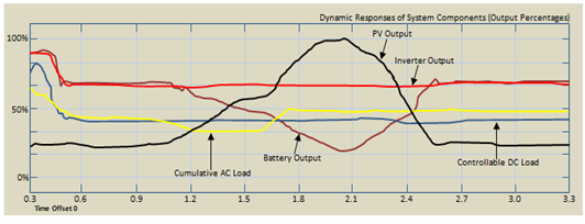
Figure 19: Graph of System Integration/Coordination

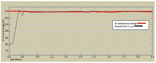
Figure 20: Graph of reference DC Link Voltage Versus the Actual DC Link Voltage

CONCLUSION

This study successfully achieved its aim of model validation for the Integrated Solar System Laboratory, ensuring accurate representation of dynamic behaviors within the integrated solar system components. Rigorous mathematical models were formulated for key components, and their implementation in MATLAB/Simulink created a virtual environment faithfully mirroring the laboratory setup. The validation process accurately mirrored designed parameters, assessing simulated outputs under varying conditions, affirming model accuracy and reliability for the integrated solar system.

A. Practical Implications

The developed system, as presented in Figure 1, demonstrates a solar energy source, battery storage, and associated controllers in a manner applicable to diverse photovoltaic solar applications. The integration of smart grid simulation, IoT connectivity, and energy management software positions it as a cutting-edge tool for practical education. The inclusion of hybrid renewable systems and energy-efficient technologies aligns with contemporary energy trends.

B. Theoretical Implications

The theoretical implications stem from the successful implementation of mathematical models for each system component. The integration of advanced control strategies, such as the incremental conductance MPPT method and inverter control in synchronous rotating reference frames, contributes to the theoretical understanding of optimizing solar energy systems.

C. Limitations

Despite the success, some limitations exist. The study primarily focuses on specific operating conditions, and the system’s response to extreme scenarios or unexpected disturbances may need further exploration. Additionally, the model’s accuracy relies on precise parameterization, and uncertainties in component characteristics may influence results.

D. Suggestions for Future Work

To enhance the study’s comprehensiveness, future work could delve into broader operational scenarios and consider additional factors like system faults and transient responses. Exploring the impact of different battery technologies and incorporating advanced machine learning algorithms for control could further refine the system’s performance. Continuous validation with real-world data under varying conditions would also strengthen the reliability of the models.

ACKNOWLEDGEMENTS

The authors gratefully acknowledge the financial support provided by the Tertiary Education Trust Fund (TETFund), Nigeria, which significantly contributed to the successful execution of this research project. Their support played a crucial role in advancing renewable energy education and fostering innovation in sustainable energy solutions.

REFERENCES

Olujobi, O. J., Okorie, U. E., Olarinde, E. S., Aina-Pelemo, A. D., (2023). Legal responses to energy security and sustainability in Nigeria’s power sector amidst fossil fuel disruptions and low carbon energy transition. Heliyon, 9(7), 1 – 24. https://doi.org/10.1016/j.heliyon.2023.e17912.
Stren & Blan Partners. (2023, November 13). Transitioning to a clean energy economy – Challenges and opportunities for Nigeria. Retrieved from https://strenandblan.com/2023/11/13/transitioning-to-a-clean-energy-economy-challenges-and-opportunities-for-nigeria/
USAID (2022). Power Africa Nigeria Power Sector Program Off-Grid Market Intelligence Report. IDIQ Contract No. 720-674-18-D-00003. Power Africa Expansion Task Order No. 720-674-18-F-00003. Power Africa Nigeria Power Sector Program (PA-NPSP). Submitted: 10 September 2021. Comments Received: 2 March 2022. Resubmitted: 1 April 2022. Approved: 19 April 2022. (pp. 9-10).
Adebanji, B., Ojo, A., Fasina, T., Adeleye, S. & Abere, J. (2022). Integration of Renewable Energy with Smart Grid Application into Nigeria’s Power Network: Issues, Challenges and Opportunities. European Journal of Engineering and Technology Research, 7(3), 18-24. DOI: http://dx.doi.org/10.24018/ejeng.2022.7.3.2792.
Piccoli, E., Dama, A., Dolara, A., & Leva, S. (2019). Experimental Validation of a Model for PV Systems under Partial Shading for Building Integrated Applications. Solar Energy, 183, 356-370. https://doi.org/10.1016/j.solener.2019.03.015.
Asim, M., Usman, M., Hussain, J., Farooq, M., Naseer, M. I., Fouad, Y., … Almehmadi, F. A. (2022). Experimental Validation of a Numerical Model to Predict the Performance of Solar PV Cells. Frontiers in Energy Research, 10, 873322, 1-15. doi: 10.3389/fenrg.2022.873322.
Herrando, M., Coca-Ortegón, A., Guedea, I., & Fueyo, N. (2023). Experimental Validation of a Solar System based on Hybrid Photovoltaic-Thermal Collectors and a Reversible Heat Pump for the Energy Provision in Non-Residential Buildings. Renewable and Sustainable Energy Reviews, 178, 1-16. doi: 10.1016/j.rser.2023.113233.
Soni, S. (2014). Solar PV Plant Model Validation for Grid Integration Studies. Master’s thesis, Arizona State University.
Jayalakshmi, N.S., Gaonkar, D.N., Balan, A., Patil, P. & Raza, S.A. (2014). Dynamic Modeling and Performance Study of a Stand-alone Photovoltaic System with Battery Supplying Dynamic Load. International Journal of Renewable Energy Research, 4(3), 635–640. https://doi.org/10.20508/ijrer.v4i3.1447.g6385.
Sultani, J. F. (2013). Modelling, Design and Implementation of D-Q Control in Single-Phase Grid-Connected Inverters for Photovoltaic Systems Used in Domestic Dwellings. (Doctoral dissertation, De Montfort University).
Haugen, F. (2005, February 17). Discrete-time Signals and Systems. TechTeach. Retrieved from http://techteach.no.
Duffie, J.A. & Beckman, W.A. (2013). Solar Engineering of Thermal Processes (4th Ed.). John Wiley & Sons, Hoboken, New Jersey. Pp 746-768.
Kremers, E., Viejo, P., Barambones, O. & Durana, J.G.D. (2010). A Complex Systems Modelling Approach for Decentralised Simulation of Electrical Microgrids. 15th IEEE International Conference on Engineering of Complex Computer Systems, Oxford, 302-311. DOI: 10.1109/ICECCS.2010.1.
Jackey, R.A. (2007). A Simple, Effective Lead-Acid Battery Modeling Process for Electrical System Component Selection. SAE Technical Paper. DOI:10.4271/2007-01-0778.
Alzahrani, A., Ferdowsi, M., Shamsi, P. & Dagli, C.H. (2017). Modeling and Simulation of Microgrid. Procedia Computer Science, 114(1), 392–400. Retrieved from: www.sciencedirect.com.
Rodriguez, L.M., Montez, C., Moraes, R. & Portugal, P. (2017). A Temperature-Dependent Battery Model for Wireless Sensor Networks. Sensors, 17(1), 422. DOI: 10.3390/s17020422.
Eckstein, J.H. (1990). Detailed Modelling of Photovoltaic Systems Components. An M. Sc. Dissertation submitted to the Postgraduate School, University of Wisconsin-Madison. Retrieved from: https://minds.wisconsin.edu/bitstream/handle/1793/45596/Eckstein.
Rauschenbach, H.S. (1980). Solar Cell Array Design Handbook: The Principles and Technology of Photovoltaic Energy Conversion. Van Nostrand Reinhold Co, New York. Pp. 332, 333, 334, 345.

Article Statistics

Track views and downloads to measure the impact and reach of your article.

PDF Downloads

506 views

Metrics

PlumX

Altmetrics

Model Validation for an Integrated Solar PV System Laboratory

ABSTRACT

INTRODUCTION

RELATED LITERATURE

METHODOLOGY

RESULTS AND DISCUSSION

CONCLUSION

ACKNOWLEDGEMENTS

REFERENCES

Article Statistics

Subscribe to Our Newsletter

Sign up for our newsletter, to get updates regarding the Call for Paper, Papers & Research.