Modeling Queuing Operational Characteristics at Automated Teller Machine Points

^*Chaku Shammah Emmanuel., Sandra Cordelia Suleiman., Awhigbo Ezekiel Bulus

Department of Statistics, Nasarawa State University, Keffi

^*Corresponding Author

DOI: https://doi.org/10.51584/IJRIAS.2024.906040 

Received: 20 March 2024; Revised: 03 April 2024; Accepted: 05 June 2024; Published: 04 May 2024

ABSTRACT

The study was designed to obtain the queuing behavior of the queuing system at a bank. The data on queuing behavior was gathered for a period of seven (7) weeks; which comprises of four (4) hours daily from 14^th August to 30^th September, 2023. Four (4) ATM machines were observed as the service discipline for the period of seven (7) weeks in the bank. Plots reveals a consistent pattern throughout the month, with Sundays and Mondays experiencing double the average customer volume compared to weekdays and Saturdays. Moving on to the operating characteristics of the system, it was observed that the average customer arrival rate is approximately 12 customers per hour, with an average service rate of 30 customers per hour. The traffic intensity (ρ) is calculated as 0.1202, indicating that, on average, 12.02% of customers keep the ATM busy per hour. The system utilization rate is 87.98%, implying that nearly 88% of customers are in the queue per hour. Additionally, the average time a customer spends in the system, considering additional transaction time, is 8.32 minutes. The probability of the system being empty is calculated as 0.389, indicating that the system is idle for 38.2% of the time and busy with customers for 61.1% of the time. Further analysis explores customer behavior, considering the probability that an arriving customer enters the system or reneges based on encountering a certain number of customers. On less busy days, an arriving customer enters the queue at 43.74% of the time, while on busy days, they enter the system at 99.97% of the time. The probability of an arriving customer reneging on less busy days is 56.26%, and on busy days, it is only 0.028%. Regarding unfairness characteristics, the system is shown to be highly discriminative.

Key words: Queuing Systems, Operations Research, ATM Queues, Service time, Arrival Time

BACKGROUND TO THE STUDY

Recently, significant reforms at efforts to maximize profit, reduce cost and satisfy customers optimally by banks are being studied. Despite these entire sterling efforts one phenomenon issues remains, queues at service points. It is a common practice to see a very long waiting line of customers to be serviced either at the Automated Teller Machine (ATM) or within the banking hall. Though similar waiting lines are seen in places like; bus stop, fast food restaurants, clinics and hospitals, traffic light, supermarket, etc. but long waiting line in the banking sector is worrisome (Abdullah et al, 2015). Queuing model analysis is largely an operations research (OR) field. It is a mathematical approach of associating customers’ arrival processes on a queue if service is not immediately accessible with their related service processes. Catalogued of queuing model applications exist in bank counters where customers await varying services; workshops where machines await repairs; warehouses where items await distributions; telephone exchange centers where incoming calls await maturation before delivery, etc. (Sharma, 2013).

A system serving a queue of people in a typical resource-oriented or service delivery environment is a microcosm social construct where emotions and resentment may develop if delay, unfairness, or injustice is practiced or perceived to be practiced in the system, whereas courtesy and even comradeship may result when fairness in service is perceived (Toshiba et al, 2013). According to recent studies, the problem of fairness in the queue system is far more important to customers than the actual delays they suffer. For example, a corporation may lose customers and/or be sued if a customer loses money as a result of being treated unfairly in line. Thus, consumers’ perception of both the fairness aspect and the quality of service rendered in a service delivery system may influence their reactions and continued patronage of an organization’s services and products (Murthy, 2014)

1.2 Statement of Problem

In the context of banking operations, the efficiency and fairness of queuing systems are paramount for ensuring a positive customer experience. Despite the crucial role of queuing systems in managing customer flow, there exists a notable gap in understanding the operational dynamics and potential sources of unfairness within these systems at banks. The current literature provides limited insights into the specific factors influencing queuing efficiency and the occurrence of unfair treatment among customers.

Efficient queuing systems are pivotal for reducing customer wait times, enhancing service quality, and ultimately improving customer satisfaction in the banking sector. However, there is a lack of comprehensive research that investigates the operational intricacies and fairness considerations within bank queuing systems. Addressing this gap is essential not only for advancing academic knowledge in queuing theory but also for providing actionable recommendations to banking institutions seeking to optimize their customer service processes.

1.3 Aim and Objectives of the study

1.3.1. Aim

The aim of this work is to study the operational and unfairness characteristic of the queuing systems at automated teller machine points.

1.3.2. Objectives

The objectives of the study are:

1. To determine the average waiting time of customers.
2. To determining the time taken to serve a customer at each service one point.

1.4 Significance of the study

This study is of immense importance to a lot of interested parties especially concerned customers of the bank who have experienced different level of queuing problem during their transactions with their banks as the information elicited from the study will help the banks management to cushion the problem of the subject matter such that. The data obtained from the field work will go a long way in assisting the board and management of these banks in making decisions about the growth of the bank. The study will also provide them with a lift to reducing the times customers spend waiting to be served.

1.5 Scope of the study

The study was designed to obtain the queuing behavior of the queuing system at Access Bank Plc, NSUK Branch Keffi, Nasarawa State. The data on queuing behavior was gathered for a period of seven (7) weeks; which comprises of four (4) hours daily from 14^th August to 30^th September, 2023. Four (4) ATM machines were observed as the service discipline for the period of forty nine (49) days lasting through seven (7) weeks in the Access Banks Plc, NSUK Branch, Keffi Nasarawa State.

METHODOLOGY 

2.1 Study area

This research methodology used in this research work is observation method. The research observed the arrival rate, service rate and departure rate at the ATM of Access Bank Plc Nasarawa State University, Keffi. The main aim of the study is to analyze the waiting line of customers at an Automated Teller Machine (ATM).

2.2 Data Collection

In this study, primary data were collected through observation. The data on queuing behavior were gathered for a period of seven (7) weeks; which comprises of four (4) hours per days of the weeks. Four (4) ATM machines were observed as the service discipline for the period of seven (7) weeks in the Access Banks Plc, NSUK Branch, Keffi Nasarawa State.

2.3 Models

2.3.1. Poisson

A Poisson queue is a queuing model in which the number of arrivals per unit of time and the number of completions of service per unit of time, when there are customers waiting, both have the Poisson distribution (Rao, 2011).

The Poisson distribution is good to use if the arrivals are all random and independent of each other. For the Poisson distribution, the probability that there are exactly x arrivals during t amount of time is:

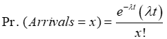
t is a duration of time. Its units are, e.g., hours or days.

λ (Greek letter lambda) is the expected (average) number of arrivals per hour, or day, or whatever units t is measured in.

λt is therefore the expected number of arrivals during t amount of time.

x is a possible number of arriving customers.

x! (“x factorial”) means 1×2×…×(x-1) × x. For example, 5! = 1×2×3×4×5. We define 0! = 1.

If arrivals are distributed according to the above formula, then we say “the arrivals are Poisson” or “have the Poisson distribution.”

2.3.2.   Exponential

If the number of events during a specified period of time has the Poisson distribution, then the amount of time between events has what is called the exponential distribution.

The Exponential Distribution:

λ is the expected number of arrivals per unit of time, as before

The Poisson and the exponential distributions are mathematically equivalent. They are two ways of looking at the same thing.

Here is an example of an exponential distribution calculation:

If λ is 1 arrival per hour, then the probability that the next arrival will be in less than 1 hour is: If λ is 1 arrival per hour, then the probability that the next arrival will be in less than 1 hour is: 1- e^-1 = 0.632.

2.4. Performance Measures of a Queuing System

The performance measures (operating characteristics) for the evaluation of the performance of an existing queuing system, and for designing a new system in terms of the level of service a customer receives as well as the proper utilization of the service facilities are listed as follows:

1. Average (or expected) time spent by a customer in the queue and system

            W_q: Average time an arriving customer has to wait in a queue before being served,

            W_S: Average time an arriving customer spends in the system, including waiting and service.

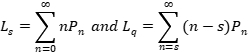
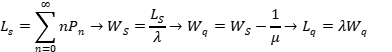
2. Average (expected) number of customers in the queue and system

            L_q: Average number of customers waiting for service in the queue (queue length)

            L_s: Average number of customers in the system (either waiting for services in the queue or beingserved).

3. Value of time both for customers and servers

           P_W: Probability that an arriving customer has to wait before being served (also called blocking probability).

: Percentage of time a server is busy serving customers, i.e., the system utilization.

P_n: Probability of n customers waiting for service in the queuing system.

P_d: Probability that an arriving customer is not allowed to enter in the queuing i.e., system capacity is full.

4. Average cost required to operate the queuing system
5. Average cost required to operate the system per unit of time
6. Number of servers (service centres) required to achieve cost effectiveness.

 (Sharma, 2016).

2.4.1. Transient-State and Steady-State

At the beginning of service operations, a, queuing system is influenced by the initial conditions, such as number of customers waiting for service and percentage of time servers are busy serving customers, etc. This initial period is termed as transient-state. However, after certain period of time, the system becomes independent of the initial conditions and enters into a steady-state condition.

To quantify various measures of system performance in each queuing model, it is assumed that the system has entered into a steady-state.

Let P_n(t) be the probability that there are n customers in the system at a particular time t. Any change in the value of P_n(t), with respect to time t; is denoted by p; (t). In the case of steady-state, we have:

 (independent of time, t)

Or

Or

If the arrival rate of customers at the system is more than the service rate, then a steady-state cannot be reached, regardless of the length of the elapsed time.

Queue size, also referred to as line length represents average number of customers waiting in the system for service.

Queue length represents average number of customers waiting in the system and being served.

Notations: The notations used for analyzing of a queuing system are as follows:

n =      Number of customers in the system (waiting and in service)

P_n =     Probability of n customers in the system

 = Average customer arrival rate or average number of arrivals per unit of time in the queuing system

 = Average service rate or average number of customers served per unit time at the place of service.

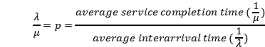 =  Traffic intensity or server utilization factor

P₀        =          Probability of no customer in the system

s          =          number of service channels (service facilities or servers).

N         =          maximum number of customers allowed in the system

L_s         =          average number of customers in the system (waiting and in service)

L_q        =          average number of customers in the queue (queue length)

W_s       =          average waiting time in the system (waiting and in service)

W_q       =          average waiting time in the queue

P_w        =          Probability that an arriving customer has to wait (system being busy), 1 — P_O = ()

For achieving a steady-state condition, it is necessary that, < 1 (i.e. the arrival rate must be less than the service rate). Such a situation arises when the queue length is limited, generally because of space, capacity limitation or customers balk.

2.4.2.   Relationships among Performance Measures

The following basic relationships hold for all infinite source queuing models.

The general relationship among various performance measures is as follows:

i) Average number of customers in the system is equal to the average number of customers in queue (line) plus average number of customers being served per unit of time (system utilization).

L_s = L_q + Customer being served

= L_q +

The value of p = — is true for a single server finite & source queuing model.

ii) Average waiting time for a customer in the queue (line)

iii) Average waiting time for a customer in the system including average service time

iv) Probability of being in the system (waiting and being served) longer than time t is given by:

and     

Where:

T = time spent in the system

t = specified time period

e = 2.718

v) Probability of only waiting for service longer than time t is given by:

vi) Probability of exactly n customers in the system is given by:

vii) Probability that the number of customers in the system, n exceeds a given number, r is given by:

The general relationships among various performance measures are:

2.5. Single-Server Queuing Models

2.5.1.   Model l: {(M/M/1): /FCFS)} Exponential Service – Unlimited Queue

This model is based on certain assumptions about the queuing system:

1. Arrivals are described by Poisson probability distribution and come from an infinite calling population.
2. Single waiting line and each arrival waits to be served regardless of the length of the queue (i.e. no limit on queue length — infinite capacity) and that there is no balking or reneging.
3. Queue discipline is ‘first-come, first-served’.
4. Single server or channel and service times follow exponential distribution.
5. Customers arrival is independent but the arrival rate (average number of arrivals) does not change over time.
6. The average service rate is more than the average arrival rate.

RESULTS AND DISCUSSION

3.1  Data presentation of weekly data collected from an ATM

The below table shows the data collected for seven weeks running through forty nine days of the study.

Table 3.1: Collected Data

	Working Days					Weekend		Weekly total
Days Weeks	Mon	Tue	Wed	Thur	Fri	Sat	Sun
	48	39	40	39	67	54	21	308
WK	33	28	41	35	49	20	16	222
WK	15	22	32	25	20	15	11	140
WK	13	17	20	18	24	39	8	139
WK	16	20	18	22	31	29	13	149
WK	21	36	19	23	32	15	17	163
WK	16	21	31	43	53	24	14	202
Monthly Total	162	183	201	205	279	196	100	1323

Source: field data, 2023.

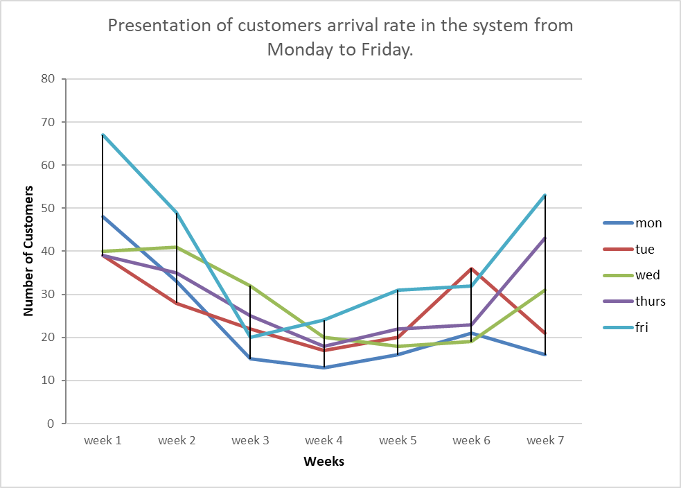
Fig. 3.1: Week day customer arrival rate on Mondays to Fridays.

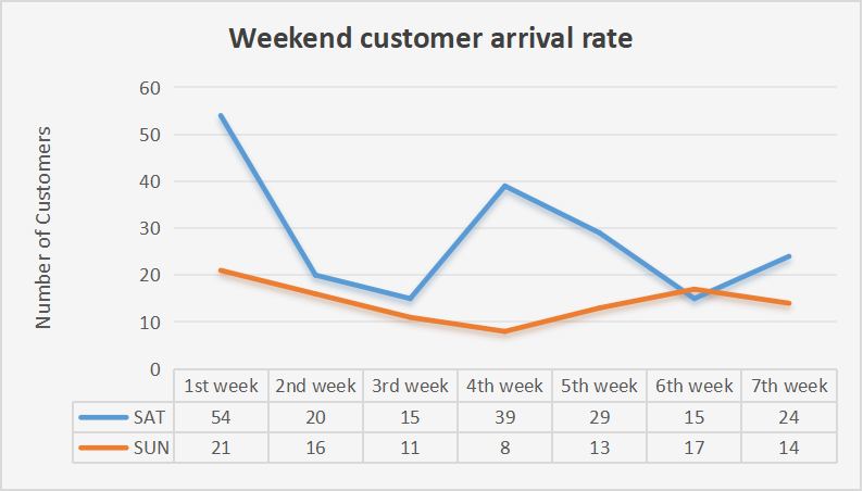
Fig.3.2: Showing the weekend customer arrival rate on Saturdays and Sundays.

Fridays and Saturdays are the busiest days of the week for the ATM servers, while the first and seventh week of the study also exhibit the highest customers traffics on the system. This may not be unconnected with the usual upsurge of customers at the ATM during the first and last week of the month where salaries are being paid while weekday’s periods also experienced high patronage on Mondays, Tuesdays and Fridays where demand for student expenses is high and also on Sunday, less people withdraw cash from the ACCESS ATM because they probably already have enough cash and most people are in doors for the weekend.

3.2  Operating Characteristic of the System.

Given that the four ATM servers run for a maximum of fourteen (14) hours per day (8am-10pm), using data from the table above where data was collected for only four (4) hours every day, the average customer’s arrival rate of the system:

Approximately that is 12 customers must arrive the system for service. From observation and discussion with the relevant security guards that an ATM knowledgeable customer spends an average of 2 minutes on the ATM machine before departure, thus, giving an average service rate:

The traffic intensity of the M/M/4 system: this gives an average of 12.02% customers per day busy ATM per hour, while the system utilization rate implies that about 87.98% of the customers are on queue per hour. If the additional time required by the customer to complete his/her services is exponentially distribution with mean , then a customer will spend an average time of 8.32 minutes from entering the system to departure. The system throughout the mean number of requests serviced per a time unit customers per hour. Thus, an average of 12 customer’s services is granted per hour. The probability that the system is empty i.e. there is no customer in the system,

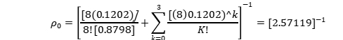
0.389

This implies that the system is always idle at only 38.2% of the time, while getting busy with customers at 1-=0.611(61.1%) of the time. We also find out that an average queue length on busy days is aboutabout 8 customers (L_q = 8). Theoretically, from Little’s theorem, the average waiting time of a customer in the queue:

W_q =  =  = 0.6667  0.7hrs = 42 minutes

The average waiting time of a customer in the system:

W_s = W_q +  = 0.7 + 0.03 = 0.73hrs = 44 minutes.

Therefore, the average number of customers in the system

L_s = W_s= 12(0.73) = 8.76  9 customers.

The probability that an arriving customer will meet k  m customers in the system:

P_k +P_o = ; k  m.

We assume that an arriving customer will join the queue if he/she meets k  m customers in the queue. Suppose the system is not empty, then an arriving customer must join the queue if it meets k  m customers in the system, otherwise he/she renege. Since the ATM’s capacity is 8 customers at any epoch, we can calculate the probability that an arriving customer meets k  8 customers in the system

Prob (a customer will enter the system) = Prob (At least one customer in queue) = Prob (At most 8 customers in the system)

P_k8 =  =  = 0.4374 = 43.74%.

Thus, on less busy days, an arriving customer will enter the queue at 43.74% of the time, or renege at 56.26% of the time. Similarly, by equation, the probability that an arriving customer will meet k  8 customers in the system are given by:

P_k = P₀= 4.075; k m

We also assume that an impatient customer will renege if he/she meets k 8 customers in the system. Suppose the maximum queue length that a patient customer can tolerate is 16 customers, since the capacity of the ATM is 8 customers at any epoch, we can calculate the probability that an arriving customer will meet at most 16 customers in the system. Therefore,

Prob (a customer will renege) = Prob (At least 8 customers in queue) = Prob (At most 16 customers in the system).

P_k8 =  = = 0.000283= 0.028%.

Thus, on busy days, an arriving customer will renege at 0.028% of the times, or enters the system at 99.97% of the times. Finally, by Erlang loss formula, the probability that an arriving customer must wait or renege (delay probability).

D = C(m,) =  =  = 0.0443

Thus, on less busy days, an arriving customer must wait for 4.43% of the time in the queue before entering into service or renege. While on the busy days, an arriving customer must wait for 95.57% of the times on queue before entering into service.

Unfairness Characteristics of the System

Given that the four parallel ATM servers run for 14 hours per day for 7 days of the week, and serve a single queue of customers on job preference policy. Therefore, the total warranted service rate of the system per day is:

(t) = 4(14) = 56 hours per day or 56- customers per day.

By equation, the momentary warranted service of each ATM machine:

 R(t) =  = 140 customers per server day.

The momentary granted rates of each ATM machine:

(t) = = 11.8125  12 customers per server day.

By equation, the momentary discrimination (deficient service) system:

(t) = 12 – 140 = -128 < 0 customers per server day.

This implies that 128 customers are dissatisfied with the bank ATM service per day.

And by equation, the accumulative discrimination (under service) of the system over its 7-day operation:

D(t) =56(16) =-896 < 0 customers per server day.

This implies that 896 customers are dissatisfied with the bank ATM service per week. Therefore, the accumulated discrimination of the 4 ATM machines over the 28 working days:

D =  = -896(28)(4) = -100,352 customers

This means a highly discriminative queuing system where 100,352 customers are dissatisfied monthly.

System Discrimination Coefficient

Let E[D²|k] for k = 0,1, 2, denote the expected value of the square of the system discrimination, given that an arriving customer encounter k customer in the system. Let P_k denote the steady state probability that there are k customers in the system. Therefore, from the “discrimination version” of the Little’s Theorem, the weekly index of the system given that an arriving customer meets k  8 customers in the system:

E[_(k)] = E[D_(k)] is given by table 3.2 below:

Table 3:2 System Discrimination with respect to  customers in System

No. of Customers	1	2	3	4	5	6	7	8	Pk8
Prob of k-Customer	0.04586	0.002267	0.00004391	0.000000516	0.0000000051	0.000000000042	0.00000000000029	0.0000000000000022	0.4374
E[(k)] = [DP(k)]	-55225.71	-2729.97	-52.87	-6.23	-6.14	-0.051	-0.0035	-0.000026	-1684307.59

The table 2.0 above shows that, given 43.74% probability that an arriving customer will meet k  8 customers on less busy days, the system discriminative index:

E[_(k)] = -1684307.59 < 0  -1684308, thus a highly discriminative system.

Similarly, the weekly discrimination index of the system, given that an arriving customer meets k  8 customers in the system is given by Table 3.3 below:

Table 3.3: System Discrimination with respect to P_{k 8} customers in System

No. of Customers	8	9	10	11	12	Pk8
Prob of k-Customer	0.00000002545	0.000000002838	0.000000000273	0.00000000000274	0.0000000000000277	0.000000028324
E[(k)] = [DP(k)]	-0.0306	-0.0034	-0.000329	-3.2995e-6	-3.3357e-8	-0.0310

The table 3.3 above shows that given 0.0000023% probability that an arriving customer will meet k8 customers in the system, the system discriminative index:

E[_(k)] = -0.0310 < 0  -0.03, thus a high discriminative system.

System Unfairness Coefficient

Let E[D²|k] for k = 0,1, 2, denote the expected value of the square of the system discrimination, given that an arriving customer encounter k customer in the system. Let P_k denote the steady state probability that there are k customers in the system, then by equation, the weekly unfairness index system, given that an arriving customer meets k  8 customers in the system is given by the table 3.4 below.

 Table 3.4: System Discrimination with respect to P_{k 8} customers in System

No. of Customers	1	2	3	4	5	6	7	8	Pk8
Prob of k-Customer	0.04586	0.002267	0.00004391	0.000000516	0.0000000051	0.000000000042	0.00000000000029	0.0000000000000022	0.4374
E[D2|kP(k)] = D2 P(k)	453962.2912	22540.9474	435.0638	5.1201	0.0505	0.0000003969	0.0000000028	0.0000000000207	476944.4756
E[D|k] P(k) = DP(k)	−4597.2432	−227.591584	−4.3990632	−0.051481632	−0.000510848	−0.000004217664	−0.000000029555968	−0.0000000002215872	−489.31054

By equation, the overall weekly unfairness, given that an arriving customer meets k8 customers in the system is:

Var[D] = E[D²]-[E[D]]² = 476,944.4756 – [−489.31054]² = 237447.963

The table 3.4 above shows that given 43.74% probability that an arriving customer will meet k8 customers on a less busy day, the system unfair coefficient Var[D] = 237447.963; thus, highly unfair system. Similarly, the weekly discrimination (unfairness) of the system given that an arriving customer meets k8 customers in the system is given by Table 3.5 below:

 Table 3.5: Unfairness Discrimination with respect to P_{k 8} customers in System

No. of Customers	8	9	10	11	12	Pk8
Prob of k-Customer	0.0000000000000022	0.000000002838	0.000000000273	0.00000000000274	0.0000000000000277	0.000000028324
E[D2|kP(k)] = D2 P(k)	0.0000000000207	0.00000028594056	0.0000000027666632	0.0000000000275704008	0.0000000000002759293568	0.0000003081933152
E[D|k] P(k) = DP(k)	−0.00000022077	−0.000283957376	−0.000027383296	−0.0000002745088	−0.000000002771904	−0.000531807232

Similarly, by equation, the overall unfairness of system given that an arriving customer meets k8 customers on the queue:

Var[D] = 0.0000003081933152 – [−0.000531807232]²

Var[D] = 0.00000002511

The table 3.5 above shows that given a 0.000028% probability that an arriving customer meets k8 customers in the queue on less busy days, the system unfairness coefficient Var[D] = 0.00000002511; also, a highly unfair system. Finally, the confidence interval (CI) for the validity/reliability of the unfairness coefficient is given by:

CI = D

Where  = 0.05 (5%)

For P_k8 customer in the system;

CI = -896  (6.314) 487.302= (−3966.9348,2174.9348)

And for P_k8 customers in the System;

CI = -896  (6.314) 0.0001585 = (−896.0006,−895.9994)

SUMMARY OF THE ANALYSIS

From the analysis so far, the summarized performance and unfairness characteristics below are typically necessary for drawing a valid conclusion and recommendations on the ATM queuing systems under consideration. Tentatively, Table 3.6 summarizes the operational characteristics while Table 3.7 represents a summary of the unfairness characteristic of the System respectively.

Table 3.6: Operational Characteristics of the System

Characteristics	Values	Characteristics	Values
Mean arrival rate, () Customers/hr	12.00	Probability that a customer renege on less busy days, %	0.028
Mean service rate, () Customers/hr	30.00	Probability that a customer enters system on less busy days, %	99.972
Traffic Intensity () %	12.02	Delay probability for less busy days, %	4.43
System Utilization, %	89.98	Delay probability for busy days %	95.57
Probability of empty system (Po) %	38.9	Mean Queue length (Lq) customers	8.0
Probability of busy server (1- Po) %	61.1	Mean Number of customers in system (Ls)	9.0
Probability that a customer enters system on less busy days, %	43.74	Mean waiting time on queue (Wq) hrs	0.7
Probability that a customer renege on less busy days, %	56.26	Mean service time in the system (Ws) hrs.	0.73

Table 3.7: Unfairness Characteristics of the system

Characteristics	Values
Total warranted service rate, (t) customers per day	560
Momentary warranted rate, R(t) customers per server day	140
Momentary granted rate, (t) customers per server day	12
Momentary discrimination, (t) customers per server day	-128
Accumulative discrimination, D(t) customers per server per week	-896
System discrimination when k  8, E[(k)] customer per week	-1684307.59
System discrimination when k  8, E[(k)] customer per week	-0.0310
System unfairness Coefficient when k  8, Var[D]	476944.4756
System unfairness Coefficient when k  8, Var[D]	0.0000003082

SUMMARY AND CONCLUSION

5.1 Summary

The background of the study introduces the concept of queuing theory and its applications, emphasizing the impact on customer behaviour and the importance of managing waiting times in service facilities. The study focuses on Access Bank Plc, NSUK Branch Keffi, Nasarawa State, using queuing models to analyse customer arrivals and waiting times.

The statement of the problem highlights the challenges faced by bank customers due to queuing issues, leading to delays, frustration, and potential disciplinary measures for employees. The study aims to address these problems and improve service delivery at Access Bank Plc.

The objectives of the study include determining inter-arrival times, average waiting times, and service times for customers. The significance of the study lies in providing valuable data for bank management to make informed decisions, reduce customer waiting times, and enhance overall service quality.

The data presented in Figure 3.1 and 3.2 reveals a consistent pattern throughout the month, Fridays and Saturdays are the busiest days of the week for the ATM servers, while the first and seventh week of the study also exhibit the highest customers traffics on the system. This may not be unconnected with the usual upsurge of customers at the ATM during the first and last week of the month where salaries are being paid while weekday’s periods also experienced high patronage on Mondays, Tuesdays and Fridays where demand for student expenses is high.

Moving on to the operating characteristics of the system, the average customer arrival rate is approximately 12 customers per hour, with an average service rate of 30 customers per hour. The traffic intensity (ρ) is calculated as 0.1202, indicating that, on average, 12.02% of customers keep the ATM busy per hour. The system utilization rate is 87.98%, implying that nearly 88% of customers are in the queue per hour. Additionally, the average time a customer spends in the system, considering additional transaction time, is 8.32 minutes.

The system’s throughput, representing the mean number of requests serviced per hour, is approximately 12 customers. The probability of the system being empty is calculated as 0.389, indicating that the system is idle for 38.2% of the time and busy with customers for 61.1% of the time.

Further analysis explores customer behavior, considering the probability that an arriving customer enters the system or reneges based on encountering a certain number of customers. On less busy days, an arriving customer enters the queue at 43.74% of the time, while on busy days, they enter the system at 99.97% of the time. The probability of an arriving customer reneging on less busy days is 56.26%, and on busy days, it is only 0.028%.

Regarding unfairness characteristics, the system is shown to be highly discriminative, with 128 dissatisfied customers per day and 896 dissatisfied customers per week. The discrimination coefficient is calculated as -100,352 customers monthly. The discrimination indices further indicate a highly discriminative system, with negative values for both scenarios of encountering fewer or more customers in the system.

The unfairness coefficient is determined to be high as well, with a weekly unfairness index of 237,447.963 for encountering fewer customers and 0.00000002511 for encountering more customers. The confidence intervals for these coefficients affirms their reliability.

5.2 Conclusion

Queuing theory plays a crucial role in understanding and improving service delivery in various industries, particularly in banking. The study at Access Bank Plc, NSUK Branch Keffi, sheds light on the queuing behavior of customers and aims to address challenges associated with delays and customer dissatisfaction.

In conclusion, the study emphasizes the importance of queuing theory in optimizing service systems, with the potential to enhance customer satisfaction and overall operational efficiency which agrees with Hung and Su (2010). The insights gained from this research can serve as a valuable resource for improving queuing management practices in Access Bank Plc and similar service-oriented organizations.

This research highlights the need for improved queue management in Access Bank Plc. Keffi branch. By analyzing customer behavior and queue performance, the bank can implement strategies to reduce waiting times, improve service quality, and enhance customer satisfaction. The study contributes to a broader understanding of queue theory and its practical applications in the banking sector.

Performance measures such as average waiting times, probabilities, and queue lengths are calculated to evaluate the efficiency of the system.

The distinction between transient-state and steady-state is crucial for accurate analysis.

The findings from these queuing models can guide improvements in the queuing system to enhance customer service and operational efficiency.

The ATM queuing system exhibits notable patterns in customer traffic and operates with characteristics that impact customer experience. The high levels of discrimination and unfairness underscore areas for improvement, suggesting that measures should be taken to enhance service delivery and reduce dissatisfaction among customers.

REFEREENCES

1. Abdullah F., Abdul W. N. and Amaresh K. (2015). A Case Study of Queuing System At ATM Machine. International Journal of Engineering Inventions e-ISSN: 2278-7461, p-ISSN: 2319-6491 Volume 5, Issue 2 PP: 07-14 ijeijournal.com.
2. Gupta, P. K. (2008). internet banking in india: consumer concern and bank strategies. Global journal of business research, 2, 43-51
3. Huang, F. and Su, L. (2010): “A study on the relationships of service fairness, quality, value, satisfaction, and loyalty among rural tourists”, 7th International Conference on Service Systems and Service Management (ICSSSM), Tokyo, June 2010, pp.1-6.
4. Ladhari, R.(2009), “Service quality, emotional satisfaction, and behavioural intentions: A study in the hotel industry”, Managing Service Quality: An International Journal, Vol. 19 No. 3, pp. 308-331. https://doi.org/10.1108/09604520910955320
5. Murthy, M. S. R., PushpaLatha, M., & KG, R. D. (2014). Minimizing The Waiting Time at Bank ATM for service with Queuing Model. International Journal of Scientific Research, 3(1).
6. Okibo A.L., Wario, B.W. (2014). Effect of e-banking on growth of customers base in Kenyan banks. http://hdl.handle.net/10419/97845
7. Rao, K. (2011). Single server Poisson queuing model with truncated exponential service times. International Journal of Mathematics and Mathematical Sciences. 7. 85-101.
8. Sanda, M.A., & Arhin, E. (2011). Using ATMs as workload relievers for Ghanaian bank tellers: the customer behavioral challenge, Journal of Economics and Behavioral Studies, 3(1), 13-21.
9. Sharma, J. K. (2013). Operations Research: Theory and Application, 5th Ed
10. Sharma, J. K. (2016). Applied Operations Research. Trinity Press. 6^th
11. Sokolov A., Veselitskaya N., Carabias V., Yildirim O. (2019) Scenario-based identification of key factors for smart cities development policies. Technological Forecasting and Social Change, vol. 148, art. 119729. Available at: https:// doi.org/10.1016/j.techfore.2019.119729, accessed 14.03.2020.
12. Tjiptono H. and Chandra, D. (2005). The effect of service quality, product excellence and promotion on consumer satisfaction cv. Primajayasarana
13. Toshiba, S., Sanjay, K.S. and Anil, K.K. (2013). A Study of Queuing Model for Banking System. International Journal of Industrial Engineering and Technology. Vol.5, No. 1 (2013), pp. 21-26