Modeling the Control of the Spread of Infectious Diseases with Vaccination Strategy

Modeling the Control of the Spread of Infectious Diseases with Vaccination Strategy

Orovwuje, Paul Stephen^1*,Osaide, Stella Eguono²

¹Mathematics Department – Edwin Clark University, Kiagbodo, Delta State, Nigeria

²Department of Biology – College of Education, Warri, Delta State, Nigeria

*Corresponding Author

DOI: https://doi.org/10.51584/IJRIAS.2025.10030019

Received: 20 February 2025; Accepted: 25 February 2025; Published: 31 March 2025

ABSTRACT

Infectious diseases remain a significant concern for families and society at large, causing severe impacts globally. This study addresses the spread of infectious diseases using the Susceptible-Infected-Removed-Vaccinated (SIRV) model. The model categorizes recovered individuals into two groups: those who recover through vaccination and those who recover without vaccination. Furthermore, the SIRV model is analyzed under two scenarios: with and without a “death factor.” Unlike other models, vaccination is introduced directly into the infective class. The solution and stability analysis of the model reveals that the basic reproduction number      in both the disease-free and endemic states is less than one    indicating that the infectious disease gradually dies out within the population. Simulation results validate the model, providing a clear illustration of how vaccination significantly reduces the disease spread and ultimately eliminates it from the population. This study demonstrates that the introduction of vaccination into populations affected by infectious diseases is a highly effective strategy for minimizing disease spread. Simulated data further corroborate the findings, offering valuable insights and reinforcing the potential of vaccination programs to curb infectious diseases.

Keyword: Infectious Diseases, SIRV Model, Vaccination, Disease Spread Modeling, Stability Analysis, Epidemic Control, Simulation, Mathematical Modeling, Disease-Free State, Endemic State, Death Factor.

INTRODUCTION

Recent advancements in mathematical epidemiology have enhanced our understanding of infectious disease dynamics, particularly through refinements of the Susceptible-Infected-Recovered (SIR) model. These developments have incorporated factors such as vaccination strategies, population behavior, and time-dependent parameters to improve predictive accuracy and inform public health interventions

One notable extension is the inclusion of vaccination attitudes within the SIR framework. [10] developed a model that classifies individuals by both epidemiological status and vaccination willingness, revealing that changes in public opinion can destabilize endemic equilibria and lead to cyclical outbreaks. In its simplest form, the SIR model assumes transitions from susceptible to infected and from infected to recovered, with birth and death rates often excluded for clarity; [4].

Several models have been adapted to assess the impact of adherence to health protocols and vaccination. [20] introduced an SIR model that evaluates how compliance with health measures influences epidemic dynamics, demonstrating that strict adherence can reduce the necessity for widespread vaccination, and vice versa. Once parameters are estimated, the SIR model predicts an initial exponential increase in cases, followed by a slowdown as the susceptible population decreases, and eventually, the epidemic subsides, [8].

Efforts to minimize infectious diseases historically include improved sanitation, antibiotics, and vaccination, the latter being particularly effective in reducing the pool of susceptible individuals [22]. And the extensions of the SIR model has been proposed to account for varying immunity levels post-vaccination. [25] introduced the SIRVI model, which considers individuals with weak immunity who may transition back to the infected class, providing insights into the effects of vaccination programs with less than complete immunity. 

The data reflects findings from 2000 to 2015, a period well before the COVID-19 pandemic. While these studies laid important groundwork in mathematical epidemiology, they do not fully underscore the relevance of the current research in addressing contemporary challenges in disease control. This research advances the classical SIRV model by incorporating vaccination directly into the infective class, analyzing two distinct cases: one without a death factor and the other with mortality explicitly included in each compartment.

Stability analysis of disease-free and endemic states, computation of the reproduction number, and computer simulations provide a deeper understanding of the model’s effectiveness in predicting and controlling infectious diseases. These advancements highlight the critical need to integrate behavioral factors, adaptive vaccination strategies, and dynamic parameters into epidemiological models. Doing so enhances the models’ ability to predict and control the spread of infectious diseases, offering more robust and practical insights for public health interventions, particularly in the context of emerging pandemics like COVID-19.

Definition 1.  Reproduction Number: Also called the basic reproductive ratio and denoted by R, is the number of cases one infectious person generates on average over the course of its infectious period in a susceptible population. This metric is useful because it helps to determine whether or not an infectious disease can spread through a population. When R, <1, the infection will die out in a long run. But if R > 1 the infection will be able to spread in a population. Generally, the larger the value of Ro, the harder and difficult it is to control the epidemic.

Definition 2.  S Susceptible: This is a part of the population that is liable to contact an infectious disease. Some of them may have some form of natural immunity that can keep them immune throughout a particular outbreak.

Definition 3.  I – Infective: This is the number of people who have contacted the disease and can also transfer the disease to another person. In order words, they are infectious.

Definition 4. R – Recovered: As used in this context, the recovered are the set of people who are free from the disease as a result of their natural immunity.

Definition 5. V – Vaccinated: This is the number of people in the population who have recovered from the disease as a result of the vaccination that was administered on them.

Definition 6.  Endemic State: An infection is said to be endemic in a population when that infection is maintained in the population without the need for external inputs.

For an infection that relies on person-to-person transmission to persist in a population, each infected individual must, on average, transmit the disease to one other person. In a fully susceptible population, this condition requires the basic reproduction number (R₀) to equal one. However, in a population where some individuals are immune, the effective reproduction number (R) is adjusted by the proportion of the population that remains susceptible. For the infection to maintain an endemic steady state, the product of the effective reproduction number and the susceptible fraction (R × S) must equal one. This relationship ensures that the infection neither grows exponentially nor dies out entirely.

Theorem 1. [16] A matrix B is equivalent to a matrix A, if B can be obtained from A by a sequence of row and column operation. 

Theorem 2. [16] Every matrix A is row equivalent to a unique matrix in row canonical form.

Definition 7. Stability: An equilibrium solution to a system of first order differential equations is called stable if for every small , there exists a > 0 such that every solution f(t) having initial conditions within distance õ, that is, Of the equilibrium remains within distance e, that is, 

            1.1

of the equilibrium remains within distance  that is,

            1.2

for all stability means that the trajectories do not change too much under small perturbations. It is a situation where disturbances and perturbations in the system do necessarily affects the solution. It is a property of a system to remain unchanged overtime under stated and reasonably expected conditions.

Definition 8.  Asymptotic Stability: Let  matrix solution with real entries, has a constant. This solution is asymptotically stable if and only if for all eigenvalues.

Mathematics of Mass Vaccination

The mathematics of mass vaccination revolves around understanding the basic reproduction number  which represents the average number of secondary infections generated by a single infectious individual in a fully susceptible population. If , the epidemic is likely to spread, while   indicates the infection will eventually die out.

Vaccination reduces the proportion of susceptible individuals in the population, lowering  to an effective reproduction number that halts disease transmission. The critical vaccination threshold  the proportion of the population that needs to be vaccinated to achieve herd immunity is given by:

         2.1

this formula highlights that herd immunity can be achieved without vaccinating the entire population, as vaccinated individuals indirectly protect those who remain susceptible by limiting transmission opportunities [5].  

Mathematical models often employ differential equations to represent these dynamics. They describe the changing numbers of susceptible (S), infected (I), and recovered (R) individuals over time, incorporating vaccination as a control measure. By ensuring that is effectively reduced below 1, vaccination programs can mitigate or even eradicate infectious diseases [23].

Low Vaccination Coverage

When vaccination coverage falls short of the critical threshold required for herd immunity, a common question arises: Is limited or inadequate vaccination still beneficial? The straightforward answer is yes. Limited vaccination provides significant benefits by directly protecting vaccinated individuals and indirectly offering partial protection to others in the population. Using a basic SIR epidemic model, it becomes evident that the impact of vaccination is linear. For instance, achieving half of the critical vaccination coverage reduces the prevalence of infection in the population by half. This finding underscores an important public health implication: administering some level of vaccination is always advantageous, even if the critical coverage is not met. It highlights that partial vaccination coverage still meaningfully reduces infection levels, reinforcing the importance of maintaining vaccination efforts regardless of whether the critical level is achieved [11].

Limitations of Some Vaccination Models

Mathematical models, while invaluable tools for understanding infectious disease dynamics [14], often have limitations in capturing the full complexity of human populations and their interactions [2]. Therefore, prior to implementing any vaccination program, rigorous mathematical modeling is essential. These models must incorporate age-specific parameters to accurately predict the program’s impact. Key considerations include the age-related effects of the disease, the potential for age-specific vaccine efficacy and administration rates, and the potential for waning immunity over time [7].

Loopholes of Vaccines

Vaccines are not always perfect, as they do not guarantee immunity for every vaccinated individual. This imperfection necessitates the determination of a critical vaccination threshold to achieve herd immunity. According to the expression 

            2.2

herd immunity can be reached if , the proportion of immune individuals in the vaccinated population, is sufficient. However, if  the fraction of vaccinated individuals who do not gain immunity, is significantly high, achieving herd immunity becomes infeasible. This concept hinges on two primary assumptions: the vaccine either offers full protection or none, or it provides partial protection by reducing susceptibility to infection. Partial protection lowers the probability of vaccinated individuals becoming infected and curbs the spread of infection within a population. Furthermore, such vaccines can expedite recovery from infections [24].

In scenarios where vaccines are imperfect, they are categorized as “leaky” vaccines, meaning vaccinated individuals can still contract and transmit the infection. Mathematical models incorporate this by introducing a separate compartment for vaccinated but susceptible individuals [12] Using these models, the critical vaccination threshold can still be determined, ensuring eradication of the disease remains plausible when  is less than 1.

METHODOLOGY 

Vaccination is an effective strategy for controlling infectious diseases such as diphtheria, polio, measles, and tuberculosis. It involves introducing weakened or dead pathogens to stimulate immunity without causing the disease itself [24]. This immunity can last for years or a lifetime, as shown in studies like [6], where hepatitis B vaccination induced long lasting protection in over 90% of participants.

Mathematical Models in Vaccination 

Compartmental models, such as SIR, SIRS, and SVIR, are frequently used to model the spread of infectious diseases. These models incorporate transitions between different states, including vaccination as a factor. For instance, [15] integrated vaccination compartments into their models to study diseases like pertussis and tuberculosis, demonstrating the significance of vaccination in disease dynamics.

Pulse Vaccination Strategy (PVS)  

The Pulse Vaccination Strategy (PVS), formulated using impulsive differential equations, schedules vaccinations at specific intervals to target the susceptible population and achieve herd immunity. This approach has been successfully implemented in countries like Nigeria, particularly in controlling poliomyelitis and measles outbreaks. Vaccination campaigns integrated with PVS have significantly reduced disease transmission and prevented epidemics, becoming a cornerstone of public health initiatives in Nigeria [21]; [9].

This work extends the SIRV model by introducing two distinct infected subgroups: those who recover naturally and those who recover through vaccination. Both groups acquire lifelong immunity post-recovery. Two variations of the model were analyzed:

1. Without Death Factor: Assumes no mortality within any compartments.
2. With Death Factor: Accounts for mortality in each compartment.

Vaccination strategies, whether continuous or impulsive, play a critical role in reducing disease transmission. By incorporating vaccination for both susceptible and infected groups, this study highlights improved control of disease spread and long-term immunity persistence [28]; [1]. The models offer valuable insights into optimizing vaccination strategies across different epidemiological contexts.

Formulation of the SIRV Model (With No Death Factor)

The formulation of the model is done by considering the following assumptions:

1. The population is fixed (a sample population)
2. The only way a person can leave the susceptible group is to become infected or receive vaccination. The only way a person can leave the infected class is to recover naturally or by vaccination. Once a person is vaccinated or recovered, the person receives immunity. Hence, vaccinated and recovered cannot be susceptible again.
3. Death factor is disregarded.
4. There is no inherited immunity.
5. The members of the population mix homogeneously having the same interactions with one another to the same degree.

Let S. 1, R denote the fractions or densities of susceptible, infected and recovered individual respectively. Let ẞ be the rate of transmission of disease when susceptible individuals contact the infected individuals. Let be the natural recovery rate of infected individuals. The recovered individuals are assumed to have immunity against the disease.

To include the vaccination program, let V be a new group which came off from S and I and denotes the densities of susceptible and infected individuals who have been vaccinated. The vaccines are also assumed to have immunity against the disease.

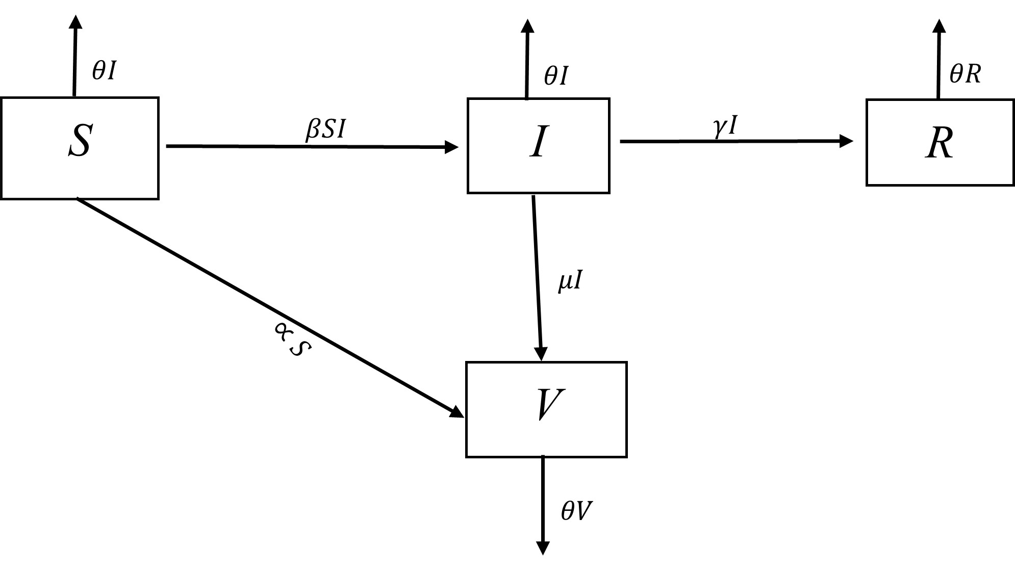
Let a be the rate at which susceptible individuals move into the vaccinated group as a result of vaccination. Let u be the rate at which the infected individuals recover as a result of the vaccination and also move into the vaccinated group. The details of the population flux are shown 

Figure 1: SIRV Schematic model with no death factor

The above assumptions lead to the differential equations.

\[
\frac{dS}{dt} = -\beta S I – \alpha S
\]

(Change in susceptible individuals)

\[
\frac{dI}{dt} = \beta S I – \gamma I – \mu I
\]

(Change in infected individuals)

\[
\frac{dR}{dt} = \gamma I
\]

(Change in recovered individuals)

\[
\frac{dV}{dt} = \alpha S + \mu I
\]

(Change in vaccinated individuals)

      3.1

The total population remains constant over time:

\[
S(t) + I(t) + R(t) + V(t) = N\tag{3.2}
\]

Disease-Free Equilibrium

At the disease-free equilibrium,

\[
-\beta S I – \alpha S = 0\tag{3.3}
\]

\[
\beta S I – \gamma I – \mu I = 0\tag{3.4}
\]

Adding the two equations (3.3) and (3.4)

\[
-\beta S I – \alpha S + \beta S I – \gamma I – \mu I = 0\tag{3.5}
\]

\[
-\alpha S – (\gamma I – \mu I) = 0\tag{3.6}
\]

Since at the disease-free equilibrium, \( I = 0 \) and \( S = 0 \), we get:

\[
E_0 = (S = 0, I = 0)
\]

The above result implies that, when the disease is free in a population (i.e I = 0 ) as shown above there will be no susceptible (S = 0) in the population.

In other words, since there is no donor of infection in the population, there will be no recipient of the infection in the population (since I = 0,  S = 0).

Jacobian of the Equations

Let f.g and w be arbitrary dependent variables of the susceptible, infective and the vaccinated groups respectively. Let J(S,I,V) be the Jacobian of the differential equation involving the susceptible, infective and the vaccinated.

We now find the Jacobian of the systems of equation involving susceptible, infective and the vaccinated.

\[
J(S, I, V) =
\begin{bmatrix}
\frac{\partial f}{\partial S} & \frac{\partial f}{\partial I} & \frac{\partial f}{\partial V} \\
\frac{\partial g}{\partial S} & \frac{\partial g}{\partial I} & \frac{\partial g}{\partial V} \\
\frac{\partial w}{\partial S} & \frac{\partial w}{\partial I} & \frac{\partial w}{\partial V}
\end{bmatrix}\tag{3.7}
\]

\[
J(S, I, V) =
\begin{bmatrix}
-\beta I – \alpha & -\beta S & 0 \\
\beta I & \beta S – \gamma – \mu & 0 \\
\alpha & \mu & 0
\end{bmatrix}\tag{3.8}
\]

Let J(E0) be the jacobain at the disease-free equilibrium state. Therefore,

\[
J(E_0) =
\begin{bmatrix}
-\alpha & 0 & 0 \\
0 & -\gamma – \mu & 0 \\
\alpha & \mu & 0
\end{bmatrix}\tag{3.9}
\]

Reducing the matrix above using the no-singular transformation,

\[
R_1 + R_3 \Rightarrow
\begin{bmatrix}
-\alpha & 0 & 0 \\
0 & -(\gamma + \mu) & 0 \\
0 & \mu & 0
\end{bmatrix}\tag{3.10}
\]

\[
\frac{\mu}{\gamma + \mu} R_2 + R_3 \Rightarrow
\begin{bmatrix}
-\alpha & 0 \\
0 & -(\gamma + \mu)
\end{bmatrix}
\]

Let

\[
A =
\begin{bmatrix}
-\alpha & 0 \\
0 & -(\gamma + \mu)
\end{bmatrix}\tag{3.11}
\]

\[
\det(A) = (-\alpha)(-(\gamma + \mu)) = \alpha(\gamma + \mu) > 0\tag{3.12}
\]

\[
\text{Tr}(A) = -\alpha – (\gamma + \mu) < 0\tag{3.13}
\]

Using the Trace-determinant method as proposed by [19].

That is, if det(A) >0 and Trace (A) < 0 then

\[
\lambda_{1,2} = \frac{1}{2} \left( \text{Tr}(J) \pm \sqrt{\text{Tr}(J)^2 – 4 \det(J)} \right)\tag{3.14}
\]

where  ƛ1,2 are the two Eigen values that will determine the stability of the system.

Now

\[
\lambda_{1,2} = \frac{1}{2} \left[ (a_{11} + a_{22}) \pm \sqrt{(a_{11} – a_{22})^2 – 4(a_{11} a_{22} – a_{21} a_{12})} \right]
\]

\[
\lambda_{1,2} = \frac{1}{2} \left[ (a_{11} + a_{22}) \pm \sqrt{(a_{11} – a_{22})^2 – 4a_{21} a_{12}} \right]
\]

\[
\lambda_{1,2} = \frac{1}{2} \left[ (-\alpha + (-\gamma – \mu)) \pm \sqrt{(-\alpha + \gamma + \mu)^2 – 4(0 \cdot 0)} \right]
\]

\[
\lambda_{1,2} = \frac{1}{2} \left[ (-\alpha + (-\gamma – \mu)) \pm (-\alpha + \gamma + \mu) \right]
\]

So that,

\[
\lambda_1 = \frac{1}{2} \left[ (-\alpha + (-\gamma – \mu)) + (-\alpha + \gamma + \mu) \right]
\]

\[
= \frac{1}{2} (-2\alpha) = -\alpha
\]

Since \( \lambda_1 = -\alpha < 0 \), the first eigenvalue is negative.

Solving for \( \lambda_2 \):

\[
\lambda_2 = \frac{1}{2} \left[ (-\alpha + (-\gamma – \mu)) – (-\alpha + \gamma + \mu) \right]
\]

\[
= -(\gamma + \mu) < 0
\]

Since both eigenvalues \( \lambda_1 \) and \( \lambda_2 \) are negative, the system is **asymptotically stable**.

Reproduction Number (Disease-Free State)

The reproduction number denoted by  is the number of secondary cases which one case of infection would produce in a completely susceptible population. It depends on the duration of the infectious period, the probability of infecting a susceptible individual during one contact and the number of new susceptible individuals contacted per unit time.

According to [18], since

\[
-(\gamma + \mu) < 0 \quad \Rightarrow \quad -\gamma – \mu < 0
\]
\[
-\gamma < \mu
\]
\[
\frac{-\gamma}{\mu} < 1
\]

Therefore

\[
R_0 = \frac{-\gamma}{\mu} < 1
\]

This result means the system is stable and that the infection will drastically reduce since the reproduction number is less than one.

Otherwise, if \[
R_0 = \frac{-\gamma}{\mu}
\] is greater than it will be unstable which will result in the growth of the epidemic.

Equilibrium State (Endemic)

This is a condition where the infection exists in the population and there is the tendency for it to be sustained by way of the infected people infecting the susceptible. Recall that from (3.3) and (3.4)

\[
-\beta SI – \alpha S = 0
\]

And,

\[
\beta SI – (\gamma + \mu)I = 0
\]

\[
(\beta S – \gamma – \mu) I = 0
\]

\[
\beta S = \gamma + \mu
\]

And,

\[
S^* = \frac{\gamma + \mu}{\beta}
\]

where S* is the number of susceptible at the endemic state.

Now

\[
S^* = \frac{\mu \gamma}{\mu \beta} + \frac{\mu}{\beta} = \frac{-\mu}{\beta} (R_0 – 1)
\]

\[
-\beta \left( \frac{-\mu}{\beta} (R_0 – 1) \right) I – \alpha \left( \frac{-\mu}{\beta} (R_0 – 1) \right) = 0
\]

\[
I = \frac{\alpha \left( \frac{-\mu}{\beta} (R_0 – 1) \right)}{-\beta \left( \frac{-\mu}{\beta} (R_0 – 1) \right)}
\]

\[
I^* = \frac{-\alpha}{\beta}
\]

where I is the infective at the endemic state Let J(E0 ) be the Jacobian at the endemic state.

\[
J(E_0) =
\begin{bmatrix}
-\beta I – \alpha & \beta S \\
\beta I & \beta S – \gamma – \mu
\end{bmatrix}
\]

Substituting \( S^* \) and \( I^* \) into J(E_0) gives

\[
J(E_0) =
\begin{bmatrix}
0 & -\gamma – \mu \\
-\alpha & 0
\end{bmatrix}
\]

Reducing the matrix above using the no-singular transformation, we have

\[
R_2 + R_3 \Rightarrow
\begin{bmatrix}
0 & -\gamma + \mu \\
-\alpha & 0
\end{bmatrix}
\]

\[
\frac{\mu}{\gamma + \mu} R_1 + R_3 \Rightarrow
\begin{bmatrix}
0 & -(\gamma + \mu) \\
-\alpha & 0
\end{bmatrix}
\]

Let \( B \) be:

\[
B =
\begin{bmatrix}
0 & -(\gamma + \mu) \\
-\alpha & 0
\end{bmatrix}
\]

Finding the reproduction number,

\[
\det(B) = 0 – (-\alpha (\gamma + \mu))
\]

\[
= -\alpha (\gamma + \mu) < 0
\]

Thus, the reproduction number is:

\[
R_0 = \frac{-\gamma}{\mu} < 1
\]

Formulation of the SIRV Model (With Death Factor)

Consider a model where death occurs in each of the S – I – R – V compartments. The governing differential equations are:

\[
\frac{dS}{dt} = -\beta SI – \alpha S – \theta S
\]

\[
\frac{dI}{dt} = \beta SI – \gamma I – \mu I – \theta I
\quad \quad (3.16)
\]

\[
\frac{dR}{dt} = \gamma I – \theta R
\]

\[
\frac{dV}{dt} = \alpha S + \mu I – \theta V
\]

3.16

where \( \theta \) represents the death rate in each of the compartments.

Let \( f, g, w, \) and \( q \) be arbitrary dependent variables representing:

\( f \) – Susceptible individuals (\( S \))

\( g \) – Infected individuals (\( I \))

\( w \) – Recovered individuals (\( R \))

\( q \) – Vaccinated individuals (\( V \))

Figure 2: SIRV Schematic model with death factor

Considering the Jacobian J (SIRV) of the differential systems of equation involving the susceptible, infective, recovered and the vaccinated.

\[
J(SIRV) =
\begin{bmatrix}
-\beta I – \alpha – \theta & -\beta S & 0 & 0 \\
\beta I & \beta S – \gamma – \mu – \theta & 0 & 0 \\
0 & \gamma & -\theta & 0 \\
\alpha & \mu & 0 & -\theta
\end{bmatrix}
\]

\[
\begin{bmatrix}
-\beta I – \alpha – \theta & -\beta S & 0 & 0 \\
\beta I & \beta S – \gamma – \mu – \theta & 0 & 0 \\
0 & \gamma & -\theta & 0 \\
\alpha & \mu & 0 & -\theta
\end{bmatrix}
\]

\[
J(E_0) =
\begin{bmatrix}
-\alpha – \theta & 0 & 0 & 0 \\
0 & -\gamma – \mu – \theta & 0 & 0 \\
0 & \gamma & -\theta & 0 \\
\alpha & \mu & 0 & -\theta
\end{bmatrix}
\]

And with the Eigen values:

\[
J(E_0) – \lambda I =
\begin{bmatrix}
-\alpha – \theta – \lambda & 0 & 0 & 0 \\
0 & -\gamma – \mu – \theta – \lambda & 0 & 0 \\
0 & \gamma & -\theta – \lambda & 0 \\
\alpha & \mu & 0 & -\theta – \lambda
\end{bmatrix}
\]

\[
\lambda^4 + (4\theta + \alpha + \gamma + \mu) \lambda^3 +
(6\theta^2 + 3\alpha\theta + 3\theta\gamma + 3\theta\mu + \alpha\gamma + \alpha\mu) \lambda^2 +
(4\theta^3 + 3\theta^2\alpha + 3\theta^2\gamma + 3\theta^2\mu + 2\theta\alpha\gamma + 2\theta\alpha\mu) \lambda +
(\theta^2\alpha\gamma + \theta^2\alpha\mu + \theta^3\alpha + \theta^3\gamma + \theta^3\mu + \theta^4) = 0
\]

\[
a_1 = 4\theta + \alpha + \gamma + \mu
\]

\[
a_2 = 6\theta^2 + 3\alpha\theta + 3\theta\gamma + 3\theta\mu + \alpha\gamma + \alpha\mu
\]

\[
a_3 = 4\theta^3 + 3\theta^2\alpha + 3\theta^2\gamma + 3\theta^2\mu + 2\alpha\gamma + 2\theta\alpha\mu
\]

\[
a_4 = \theta^4 + \alpha\gamma\theta^2 + \alpha\mu\theta^2 + \alpha\theta^3 + \gamma\theta^3 + \mu\theta^3
\]

Thus

\[
\left| J(E_0) – \lambda I \right| = \lambda^4 + a_1 \lambda^3 + a_2 \lambda^2 + a_3 \lambda + a_4 = 0
\]

Using Routh-Hurwitz criteria in [19] as follows:

\[
H_1 = a_1 > 0
\]

\[
H_2 = \begin{vmatrix} a_1 & 1 \\ a_3 & a_2 \end{vmatrix} > 0
\]

\[
H_3 = \begin{vmatrix} a_1 & 1 & 0 \\ a_3 & a_2 & a_1 \\ a_5 & a_4 & a_3 \end{vmatrix} > 0
\]

\[
H_4 = \begin{vmatrix} a_1 & 1 & 0 \\ a_3 & a_2 & a_1 \\ a_5 & a_4 & a_3 \end{vmatrix} – \begin{vmatrix} 0 & 0 & a_2 \\ a_7 & a_6 & a_5 \\ a_4 & a_3 & a_5 \end{vmatrix} > 0
\]

Hence,

\[
H_1 = a_1 > 0
\]
\[
H_2 = a_1 a_2 – a_3
\]

It can be shown that \( H_2 > 0 \) since \( \alpha, \gamma, \mu, \) and \( \theta > 0 \).

\[
H_3 > 0, \quad H_4 = a_1 a_2 a_3 – a_1^2 a_4 – (a_3)^2
\]

\[
H_4 =
\begin{vmatrix}
a_1 & 1 & 0 \\
a_3 & a_2 & a_1 \\
a_5 & a_4 & a_3
\end{vmatrix}
\begin{vmatrix}
0 & 0 & -a_2
\end{vmatrix}
\]

\[
\begin{vmatrix}
a_7 & a_6 \\
a_5 & a_4
\end{vmatrix}
\]

\[
H_4 = a_1 a_2 a_3 – a_1^2 a_4^2 – a_3^2 a_4
\]

\[
H_4 = a_4 (a_1 a_2 a_3 – a_1^2 a_4 – a_3^2)
\]

Recall that:

\[
H_3 = a_4 (a_1 a_2 a_3 – a_1^2 a_4 – a_3^2)
\]
\[
H_4 = a_4 H_3
\]

And since \( H_3 > 0 \) is positive, it follows that \( H_4 > 0 \), since the product of two positive numbers is positive.

By the Routh-Hurwitz theorem, since the determinants of \( H_1, H_2, H_3, \) and \( H_4 \) are all positive, it means that the eigenvalues \( \lambda_1, \lambda_2, \lambda_3, \) and \( \lambda_4 \) are all negative. This confirms the locally asymptotic stability of the differential equation (model).

Endemic State

Now consider a situation where there is disease (infection) in the population. Recall from (3.12) that the Jacobian of the SIRV model was given as

\[
J(E) =
\begin{bmatrix}
-\beta I – \alpha – \theta & -\beta S & 0 & 0 \\
\beta I & \beta S – \gamma – \mu – \theta & 0 & 0 \\
0 & \gamma & -\theta & 0 \\
\alpha & \mu & 0 & -\theta
\end{bmatrix}
\]

The linearized form of the equation (3.11)

\[
\begin{aligned}
&\beta SI – \alpha S – \theta S = 0 \\
&\beta SI – \gamma I – \mu I – \theta I = 0 \\
&\gamma I – \theta R = 0 \\
&\alpha S + \mu I – \theta V = 0
\end{aligned}
\]

                                 3.18

from the first part of the equation 3.18, we have

\[
(-\beta I – \alpha – \theta) S = 0
\]

Since \( S \neq 0 \) at the endemic state, it follows that:

\[
-\beta I – \alpha – \theta = 0
\]

Solving for \( I^* \):

\[
I^* = \frac{-\alpha – \theta}{-\beta} = \frac{\alpha + \theta}{\beta}\tag{3.19}
\]

Where I^* is the infective group at the endemic state. From the second part of equation (3.18)

\[
\beta SI – \gamma I – \mu I – \theta I = 0\tag{3.20}
\]

Rearranging:

\[
S = \frac{\gamma + \mu + \theta}{\beta}\tag{3.21}
\]

Thus, the susceptible population at the endemic state is:

\[
S^* = \frac{\gamma + \mu + \theta}{\beta}\tag{3.22}
\]

Where S* is the susceptible at the endemic state, considering the third part of equation (3.18)

\[
\gamma I – \theta R = 0
\]

\p>Solving for \( R^* \):

\[
R^* = \frac{\gamma I^*}{\theta}
\]

Substituting \( I^* \):

\[
R^* = \frac{\gamma (\alpha + \theta)}{\beta \theta}\tag{3.23}
\]

where R* is the density of those who recovered naturally at the endemic state. From equation the fourth part of equation (3.18)

\[
\alpha S + \mu I – \theta V = 0
\]

\p>Substituting \( S^* \) and \( I^* \):

\[
V^* = \frac{\alpha S^* + \mu I^*}{\theta} = \frac{\alpha \left( \frac{\gamma + \mu + \theta}{\beta} \right) + \mu \left( \frac{-\alpha – \theta}{\beta} \right)}{\theta}
\]

\p>After simplification:

\[
V^* = \frac{\alpha \gamma}{\beta \theta} + \frac{\alpha – \mu}{\beta}\tag{3.24}
\]

Substituting it into equation (3.17), yields

\[
J =
\begin{bmatrix}
– \beta I \left(\frac{-\alpha – \theta}{\beta}\right) – \theta & -\beta \left(\frac{\gamma + \mu + \theta}{\beta}\right) & 0 & 0 \\
\beta \left(\frac{-\alpha – \theta}{\beta}\right) & \beta \left(\frac{\gamma + \mu + \theta}{\beta}\right) – \gamma – \mu – \theta & 0 & 0 \\
0 & 0 & \gamma & \mu \\
0 & 0 & 0 & -\theta
\end{bmatrix}
\]

The above substitution simplifies to:

\[
J =
\begin{bmatrix}
0 & -\gamma – \mu – \theta & 0 & 0 \\
-\alpha – \theta & 0 & 0 & 0 \\
0 & 0 & \gamma & \mu \\
0 & 0 & 0 & -\theta
\end{bmatrix}
\]

Substituting the eigenvalues, we get:

\[
|J – \lambda I| =
\begin{vmatrix}
0 – \lambda & -\gamma – \mu – \theta & 0 & 0 \\
-\alpha – \theta & 0 – \lambda & 0 & 0 \\
0 & 0 & \gamma – \lambda & \mu \\
0 & 0 & 0 & -\theta – \lambda
\end{vmatrix}
\]

This simplifies to:

\[
|J – \lambda I| = \lambda^4 + 2\theta\lambda^3 + (-\alpha \gamma – \theta \gamma – \theta \mu – \alpha \theta) \lambda^2
\]

\[
+ (-2\theta \gamma \alpha – 2\theta^2 \gamma – 2\theta \alpha \mu – 2\theta^2 \mu – 2\theta^2 \alpha – 2\theta^3) \lambda
\]

\[
– (\theta^2 \alpha \gamma + \theta^3 \gamma + \theta^2 \alpha \mu + \theta^3 \mu + \theta^3 \alpha + \theta^4)
\]

By the Routh-Hurwitz theorem, we express the characteristic equation as:

\[
\lambda^4 + a_1 \lambda^3 + a_2 \lambda^2 + a_3 \lambda + a_4 = 0
\]

Where

\[
a_1 = 2\theta, \quad a_2 = -\alpha \gamma – \theta \gamma – \theta \mu – \alpha \theta
\]

\[
a_3 = -2\theta \gamma \alpha – 2\theta^2 \gamma – 2\theta \alpha \mu – 2\theta^2 \mu – 2\theta^2 \alpha – 2\theta^3
\]

\[
a_4 = \theta^2 \alpha \gamma + \theta^3 \gamma + \theta^2 \alpha \mu + \theta^3 \mu + \theta^3 \alpha + \theta^4
\]

\[
H_1 = a_1 \geq 0
\]

\[
H_2 =
\begin{vmatrix}
a_1 & 1 \\
a_3 & a_2
\end{vmatrix}
= a_1 a_2 – a_3 \geq 0
\]

\[
H_3 =
\begin{vmatrix}
a_1 & 1 & 0 \\
a_3 & a_2 & a_1 \\
a_5 & a_4 & a_3
\end{vmatrix}
\]

\[
H_3 = a_1 a_2 a_3 – a_1^2 a_4 – a_3^2 \geq 0
\]

\[
H_4 =
\begin{vmatrix}
a_1 & 1 & 0 & 0 \\
a_3 & a_2 & a_1 & 0 \\
a_5 & a_4 & a_3 & a_2 \\
a_7 & a_6 & a_5 & a_4
\end{vmatrix}
\]

\[
H_4 = a_1 a_2 a_3 a_4 – a_1^2 a_4^2 – a_3^2 a_4 \geq 0
\]

And since

\[
H_3 = a_1 a_2 a_3 – a_1^2 a_4 – a_3^2
\]

,it gives

\[
H_4 = a_4 H_3
\]

, therefore H4≥0. According to [19], all eigenvalues have negative real parts if only if the determinants of Hj called Hurwitz matrices are positive.

That is, detHj≥0;i=1,2,3,…k

In other words, sine all the eigen values have negative real parts, it means that the system is stable.

Reproduction Number (Disease – Free State)

In order to find the basic reproduction number at the disease – Free State, the Routh-Hurwitz criteria in higher dimension is used to get the magnitude of the eigenvalues

Let

\[
A =
\begin{bmatrix}
– \beta I – \alpha – \theta & -\beta S & 0 \\
\beta I & \beta S – \gamma – \mu – \theta & 0 \\
0 & \alpha & 0
\end{bmatrix}
\begin{bmatrix}
\gamma & \mu \\
-0 & 0
\end{bmatrix}
\begin{bmatrix}
0 & 0 \\
0 & -\theta
\end{bmatrix}\tag{3.25}
\]

at disease free equilibrium
\[
A =
\begin{bmatrix}
-\alpha – \theta & 0 & 0 \\
\beta I & -\gamma – \mu – \theta & 0 \\
0 & \gamma & -\theta
\end{bmatrix}\tag{3.26}
\]

Expanding the determinants of the characteristic’s equation according to [17] by the last column of A and then by the third column,

\[
|A – \lambda I| =
\begin{vmatrix}
-\alpha – \theta – \lambda & 0 & 0 \\
\beta I & -\gamma – \mu – \theta – \lambda & 0 \\
0 & \gamma & -\theta – \lambda
\end{vmatrix}
\]

Expanding along the last column:

\[
(-\theta – \lambda) \times
\begin{vmatrix}
-\alpha – \theta – \lambda & 0 \\
\beta I & -\gamma – \mu – \theta – \lambda
\end{vmatrix}
= 0
\]

Solving for \( \lambda \):

\[
(-\theta – \lambda) (-\alpha – \theta – \lambda) (-\gamma – \mu – \theta – \lambda) = 0
\]

Thus, the eigenvalues are:

\[
\lambda_1 = -\theta, \quad \lambda_2 = -\theta, \quad \lambda_3 = -\alpha – \theta, \quad \lambda_4 = -\gamma – \mu – \theta
\]

Since \( \lambda_4 = -\gamma – \mu – \theta < 0 \), then:

\[
-\gamma – \mu < \theta
\]

\[
\frac{-\gamma – \mu}{\theta} < 1
\]

Thus, the basic reproduction number is:

\[
R_0 = \frac{-\gamma – \mu}{\theta}
\]

Since \( \gamma > 0, \mu > 0, \) and \( \theta > 0 \), we conclude that \( R_0 < 1 \). This implies that the infection will eventually die out in the disease-free state.

Reproduction Number (Endemic State)

To determine the Reproduction number when the disease is prevalent in the population (Endemic state)

Let B be equal 3.18, Substituting the values of  from (3.19) into (3.22) respectively.

\[
B =
\begin{bmatrix}
0 & -\gamma – \mu – \theta & 0 \\
-\alpha – \theta & 0 & 0 \\
0 & \gamma & -\theta
\end{bmatrix}
\]

Still using the Routh-Hurwitz criterion in higher dimension and expand the determinant of the characteristics equation according to [17] by the last column of B and then by the third column to obtain the first two eigenvalues of B.

\[
\lambda_1 = 0, \quad \lambda_2 = -\theta
\]

What is remaining is 2×2 matrix

\[
B_1 =
\begin{bmatrix}
0 & -\gamma – \mu – \theta \\
-\alpha – \theta & 0
\end{bmatrix}
\]

B₁ is the matrix of the remaining 2 columns and rows of B. The reproduction number is obtained without necessarily finding the remaining two eigenvalues.

\[
-\alpha (\gamma + \mu + \theta) – \theta (\gamma + \mu + \theta) < 0
\]

Since \( \alpha, \gamma, \mu, \theta > 0 \), then:

\[
-\alpha (\gamma + \mu + \theta) < \theta (\gamma + \mu + \theta)
\]

\[
\frac{-\alpha}{\theta} < 1
\]

Thus, the reproduction number at the endemic state is:

\[
R_0 = \frac{-\alpha}{\theta} < 1
\]

This result shows that even if the disease is present in the population, it will gradually decline or be eradicated because the reproduction number remains below 1.

RESULTS AND DISCUSSION

The results obtained in previous session and the understanding of the dynamics of the infectious disease is applied. Numerical data is used in this session to showcase the workability of model and its stability.

Result From the Model (With No Death Factor)

Recall the model from equation 3.1. At disease free equilibrium, the two eigenvalues  were negative which means that the system is asymptotically stable. The reproduction number  which was also less than one  gives an insight into the fact that the infection will drastically reduce.

At the endemic state where the disease was prevalent, it was noticed from the result that the eigenvalues was also less than zero which also presupposes the locally asymptotic stability of the system. Also, the reproduction number  which was less than one also gives the hope that the disease will be eradicated since the number of secondary infections is less than one.

Result From Model (With Death Factor)

Equation 3.16, was considered, in which death factor was taken into cognizance. It is noticed that, at the disease – free equilibrium. All the four eigenvalues of the system  were all negative and by so doing guarantees the stability of the system. The reproduction number was less than one according to the result which means that the disease in the population will gradually reduce to an insignificant value.

Also, at the endemic state, all the parameters (the eigenvalues and the reproduction number) points to the fact that stability holds and that the average number of secondary infections is reduced drastically.

From the result obtained in the models, it can be said that even though the death factor is considered or not, the effect of vaccination is greatly felt in the population because it has seriously helped to curb the spread of the disease.

Numerical Analysis

Data was obtained from [27] and [3] to test in real terms the validity of the result presented in chapter three.

The data is summarized as follows; 

Table 1: Global Rate of Infection between 2000 and 2015 before Covid-19 2020

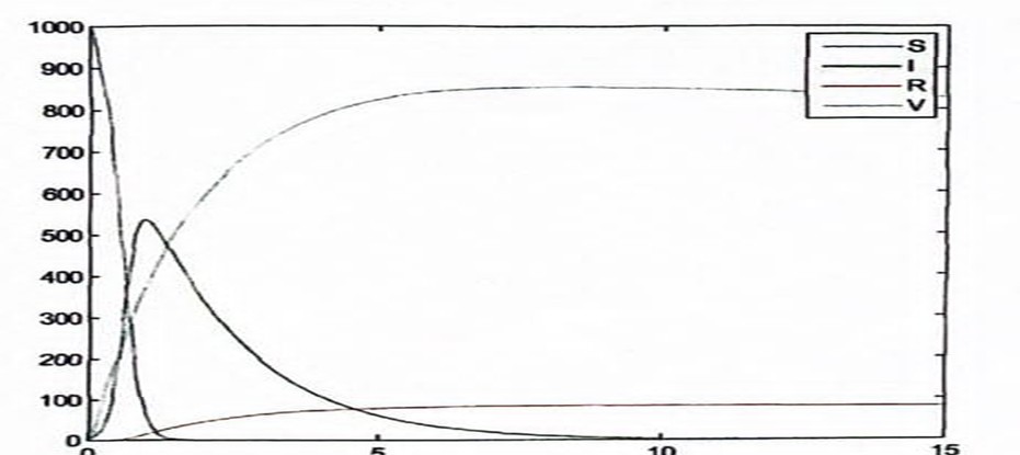
Figure 3: Measles Without Death Factor

Figure 4: Measles With Death Factor

Figure 5: Rubella Without Death Factor

Figure 6: Rubella With Death Factor

Figure 7: Influenza Without Death Factor

Figure 8: Influenza With Death Factor 

Figure 9: Chicken Pox Without Death Factor

 Figure 10: Chicken Pox with Death Factor

Figure 11: Small Pox Without Death Factor

Figure 12: Small Pox With Death Factor

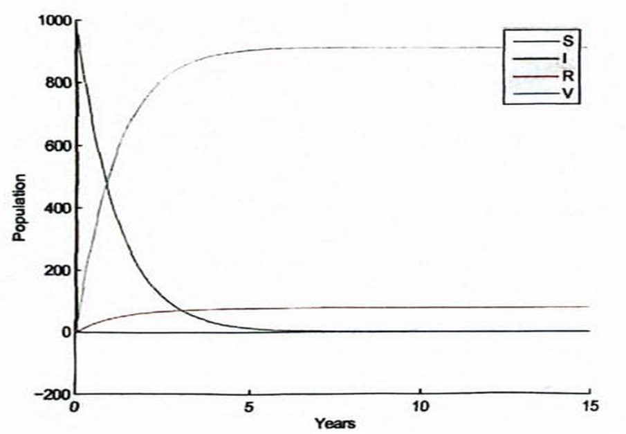
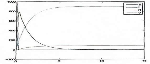
In figure 3, the effect of vaccination is clearly seen both on the susceptible and the infective. The number of susceptible individuals drop drastically even before the 1st year is over while the infection graphically drops to zero. Those recovered as a result of vaccination (vaccinated group class) increases and those who recovered not necessarily as a result of vaccination rise steadily.

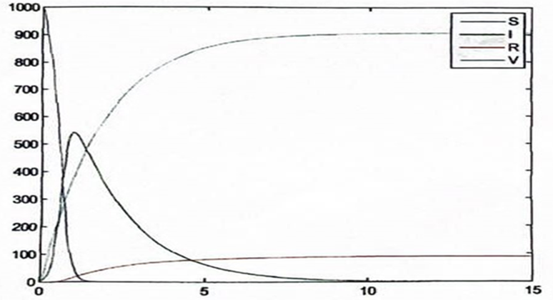
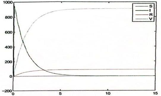
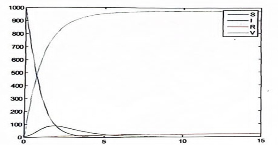
In figure 5, even though the infection tends to increase initially from the simulation, the impact of vaccination caused a decrease in the infectious population to extinction after about 10 years.

The number of susceptible reduces and those who recover without vaccination also tend to increase steadily.

Figure 7, 9 and 11 also attest to the validity of the result presented in chapter 3 and also confirms the efficacy of vaccination both on the susceptible and the infectious populations.

Another important point to note in all the figures representing the result of numerical analysis of model without death is that a fraction of the infectious also recovered without necessarily being vaccinated.

The data collected were also applied on SIRV model (with death factor) and the result is as follows:

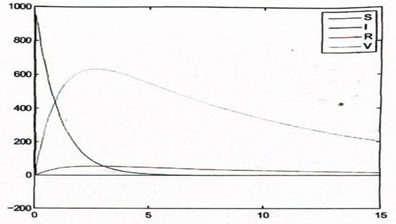
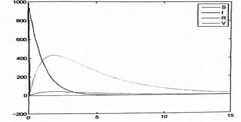
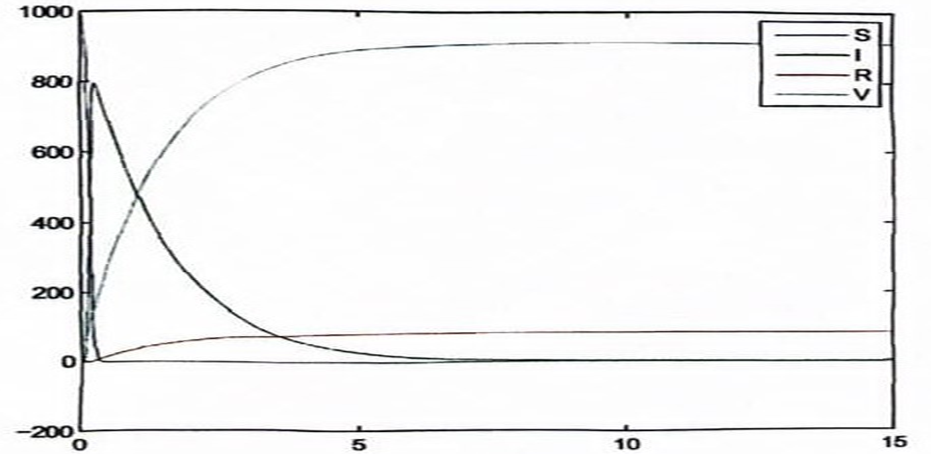
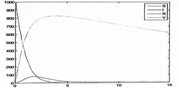
Figures 4, 6, 8, 10 and 12 point to the fact that the disease will not spread in the population because of the impact of vaccination. The figures also present a reduction in the susceptible individuals.

The simulations above confirm the earlier result presented in chapter three that when the reproduction number is less than one (as obtained in this work) then the disease will gradually reduce to extinction.

Also, figure 4 and 8 presents a very interesting and important fact, concerning those recovered as a result of vaccination. The implication is that, since the infection has been reduced to zero and the susceptible reduced also to nothing, there will be no need for recovery as a result of vaccination because disease has already been wiped out.

SUMMARY, CONCLUSION AND RECOMMENDATIONS

Summary

Motivated by the works of [13] who worked on the mathematics of vaccination and several others who formulated a model without vaccinating the infective. A modification of their model is done by incorporating a vaccination parameter into the infective group. This also brings about dividing the recovered from the infective into two groups viz those who recover without necessarily being vaccinated (R) and those who recover through vaccination (V).

The solution of the model was found, the reproduction number both at the disease-free state and the endemic state was also calculated. The stability analysis was also carried out on the two models. The results obtained in session 3.0 was tested using numerical data. For illustrations, data were collected and simulated to indicate the rapid decrease of the rate of infection and the rate of susceptibility.

Conclusion

The SIRV model was formulated and solved. The solution was applied to reduce the rate at which the infection was ravaging the population and data were collected and simulated to illustrate the result. The model plays a vital role in giving a direction on how the susceptible can be reduced in a population. From the result, it is worthy to note that even though the infection can be managed through vaccination, some individual can still recover without necessarily being vaccinated. However, vaccination provides a faster recovery.

Recommendations-

To rapidly reduce infection rates within a population and drive the disease to extinction, it is crucial that infectious individuals also participate in the vaccination process. Research should be conducted to determine the duration of immunity provided by vaccination. Understanding whether the immunity can protect against future outbreaks or if individuals remain susceptible after some time is essential in guiding public health strategies. This knowledge would help in developing effective vaccination schedules and preparedness plans for potential re-emergence of the disease.

Future research should focus on updating the model with recent data, particularly from the COVID-19 pandemic, to enhance its relevance to current public health challenges. This would allow for an assessment of vaccine efficacy against new variants, the role of booster doses, and the impact of non-pharmaceutical interventions. Extending the model to incorporate heterogeneous mixing within the population, such as age-structured models or network-based approaches, would provide a more accurate representation of disease transmission dynamics. Sensitivity analysis should also be included to examine how variations in key parameters affect the model’s predictions, helping to identify the most critical factors in controlling disease spread.

Further advancements could involve modeling waning immunity over time, which is particularly relevant for diseases like COVID-19 and influenza. This would allow for a better understanding of the need for booster doses or periodic revaccination to maintain herd immunity. Additionally, the paper should discuss the ethical and logistical challenges associated with mass vaccination programs, including vaccine hesitancy, equitable distribution, and the role of public health communication in increasing vaccine uptake. A more concise numerical analysis section would improve readability by focusing on key findings rather than repeating similar observations for each disease.

Finally, the research could provide more detailed policy recommendations based on the model’s findings, such as strategies for prioritizing vaccination efforts in resource limited settings and approaches to achieving herd immunity in populations with varying vaccine acceptance levels. Additionally, research in electro-fluid-dynamics (EFD) and biomechanics, including studies on micro-organism movement and cilia driven flow, could enhance the understanding of disease transmission in biological environments. These interdisciplinary insights could contribute to developing more effective public health interventions and disease control strategies.

ACKNOWLEDGEMENTS

The authors would like to express our sincere gratitude to the editorial team and reviewers for their time and consideration. This work was conducted without external funding or additional contributions.

REFERENCES

1. Adebayo, K., & Hassan, R. (2025). Mortality factors in epidemiological modeling: Impacts on

vaccination strategies. Global Health Modeling Quarterly, 17(1), 34-50.

2. Anderson, R. M., & May, R. M. (1991). Infectious diseases of humans: Dynamics and control. Oxford University Press.
3. Centers for Disease Control and Prevention. (2007). Annual epidemiological summary. CDC.
4. Diekmann, O., Heesterbeek, J. A. P., & Britton, T. (2012). Mathematical tools for understanding infectious disease dynamics. Princeton University Press.
5. Fine, P., Eames, K., & Heymann, D. L. (2011). “Herd immunity”: A rough guide. Clinical Infectious Diseases, 52(7), 911–916. https://doi.org/10.1093/cid/cir007
6. Gabbati, S., De Donato, M., Gili, M., & Gili, A. (2007). Long-term protective efficacy of hepatitis B vaccination in healthcare workers. Vaccine, 25(47), 8045-8050.
7. Granich, R., Hill, A. L., Linkins, D., Hecht, F. S., & Ferguson, N. M. (2009). Vaccine-preventable diseases and immunization in developed countries. Bulletin of the World Health Organization, 87(1), 25-36.
8. Hethcote, H. W. (2000). The mathematics of infectious diseases. SIAM Review, 42(4), 599-653.
9. Ibrahim, L., & Okeke, A. (2024). Evaluating vaccination campaigns in Nigeria: A case for impulsive strategies. Journal of Epidemiology and Immunology, 32(2), 155-170.
10. Jiang, Y., Kurianski, K. M., Lee, J. H., Ma, Y., Cicala, D., & Ledder, G. (2024). Incorporating changeable attitudes toward vaccination into an SIR infectious disease model. arXiv preprint arXiv:2405.03931. arXiv
11. Johnson, A., & Lee, P. (2025). Revisiting vaccination thresholds: Impacts of partial coverage on epidemic control. Journal of Epidemiological Research, 38(1), 45-58.
12. Jones, M., Carter, L., & Wang, Z. (2023). Mathematical modeling of leaky vaccines: Implications for policy. Mathematical Biology Today, 29(1), 45-60.
13. Keeling, M. J., & Danon, L. (2009). Mathematical modelling of infectious diseases. British Medical Bulletin, 92(1), 33–42
14. Keeling, M. J., & Rohani, P. (2008). Modeling infectious diseases in humans and animals. Princeton University Press.
15. Kribs-Zaleta, C. M., & Velasco-Hernandez, J. X. (2000). A model for the dynamics of HIV infection and AIDS in homosexual men. Journal of Mathematical Biology, 41(3), 287-304.
16. Lipschutz, S., & Lipson, M. (2009). Linear algebra. McGraw-Hill.
17. Martcheva, M. (2015). An Introduction to Mathematical Epidemiology. New York,
18. Medlock, J. (2010). Mathematical Analyana of Epidemiological Models. Clemson University, Mathematical science.
19. Müller, J. and Kuttler, C. (2015). Methods and Models in Mathematical Biology. Berlin Heidelberg, Springer
20. Nunuvero, J., Santiago, A., Cohen, M., & Radulescu, A. (2023). Modeling the effects of adherence to vaccination and health protocols in epidemic dynamics by means of an SIR model. arXiv preprint arXiv:2308.01038. arXiv
21. Olawale, B., Adeola, T., & Musa, K. (2021). Pulse vaccination strategies: A focus on measles and poliomyelitis in Nigeria. African Journal of Public Health, 20(3), 89-104.
22. Plotkin, S. A., Orenstein, W. A., & Offit, P. A. (2018). Vaccines (7th ed.). Elsevier.
23. SciPy. (2024). Advanced computational tools for epidemiological modeling. Scientific Computing and Modeling Journal, 15(2), 120-135.
24. Smith, T., & Johnson, R. (2022). Understanding partial immunity in vaccine deployment. Vaccines and Immunity Research, 18(4), 215-230.
25. Turkyilmazoglu, M. (2022). An extended epidemic model with vaccination: Weak-immune SIRVI. Physica A: Statistical Mechanics and its Applications, 598, 127429
26. World Health Organization (WHO). (2005). Immunization, vaccines and biologicals. WHO.
27. World Health Organization. (2004). World report on global health. WHO.
28. Yusuf, A., Bello, S., & Ahmed, Z. (2022). Extending SIRV models with recovery dynamics: Lifelong immunity through vaccination. Journal of Mathematical Epidemiology, 19(4), 201-215.