
Process Parameter Influence on Chitin Yield from Tilapia Fish Scales: A Statistical Approach
- Akinbomi, J. G.
- Abdulkareem, Y. T.
- Adesina, A.A
- Aminu, K. A
- Bakare, L
- 184-198
- Mar 27, 2025
- Education
Process Parameter Influence on Chitin Yield from Tilapia Fish Scales: A Statistical Approach
Akinbomi, J. G.*, Abdulkareem, Y. T., Adesina, A.A., Aminu, K. A., Bakare, L.
Department of Chemical Engineering, Faculty of Engineering, Lagos State University, Epe Campus, Epe, Lagos State, Nigeria
*Corresponding Author
DOI: https://doi.org/10.51584/IJRIAS.2025.10030013
Received: 11 March 2025; Accepted: 18 March 2025; Published: 28 March 2025
ABSTRACT
The extraction of valuable resources from waste materials, including chitin, is a crucial element of sustainable development. Despite the availability of chitin in abundant supply in nature, it remains largely untapped due to chitin materials being considered, generally, as waste. Therefore, this study investigated the effective extraction of chitin from tilapia fish scale waste for future valorisation of the chitin waste. The experimental runs and optimization were determined using Central Composite Design (CCD) of Response Surface Methodology (RSM) in Design Expert software with four experimental factors for chitin production. Demineralization and deproteinization using HCl (0.5 – 6.5 M) and NaOH (0.5 – 2.5 M), respectively led to the production of the chitin. The agreement between the Predicted R² (0.9666) and the Adjusted R² (0.9888) suggests high consistency and reliability of the model predictions. The optimal product was achieved at 1M HCl for 12 hours demineralization, 1M NaOH, and 2 hours deproteinization to produce Chitin. The sample of Chitin produced shows a single band for amide I at 1652 cm-1 (amide I) representing C= O stretching vibrations, and another at 1543 cm-1 (amide II) indicating N-H bending and C-N stretching vibrations, confirming the presence of β-chitin. The morphology showed that the chitin is porous and fibrous. The moisture content, ash content, bulk density and pH being 9.6%, 3.1%, 0.15 g/ml and 7.2, respectively.
Keywords – Chitin, Waste, Extraction, Optimization, Valorisation
INTRODUCTION
Chitin (C8H13O5N)n is a fibrous polymer of N-acetyl-glucosamine, an amide derivative of glucose, that is found in abundant quantity in nature, and exists as a basic cell wall component of many fungi, insect exoskeletons, and crustacean shells [1,2]. Annually, living organisms produce a substantial amount of waste including chitin, estimated to be around 8-10 billion tons [3]. Despite this vast amount of chitin, it remains largely untapped due to chitin resources being generally considered as waste [4]. The urgent need for valorising vast amount of chitin wastes cannot be understated because of the wide range of applications of chitin various industries. The exceptional properties of chitin, which make them essential components in the external protective structures of living systems, are now being extensively explored and utilized in various significant research fields, including, pulp and paper, textiles, medical applications, cosmetics, biotechnology, agriculture, food industries, chemical production, separation processes, and environmental applications [5].
To fully utilize chitin as an advanced material on a global scale, it is essential to implement effective waste management strategies and develop protocols for industrial-scale isolation and purification. On a large scale, chitin is often extracted from crab, shrimp, shellfish or lobster shells; and is used for various applications including for medical and biotechnological purposes [6, 7] including, induction of plant defence mechanisms [8]; soil conditioning to enhance crop productivity [9]; and food thickening and stabilization [10]. Chitin, which holds significant value as a lightweight and strong resource, is structurally comparable to cellulose, and functionally comparable to keratin. Chitin is semi-crystalline and has three polymorphic forms, including α -, β -, and γ -chitin. Polysaccharide α -chitin is the most common, in which the chains of a-chitin are arranged in an anti-parallel manner with strong intermolecular hydrogen bonding. β -Chitin chains are parallel to each other, with relatively weak intermolecular hydrogen bonding. Chains of γ -chitin are a mixture of α – and β chitin, with two parallel chains in one direction and a third one in the opposite direction [11].
One promising potential source for chitin material is the tilapia fish scale [12], which is abundantly generated as waste in both aquaculture and seafood processing industries. The tilapia fish, is a well-known freshwater fish that exhibits rapid growth and remarkable adaptability to diverse environmental conditions. The fish scale, serving as a protective covering, is primarily composed of chitin, making it an excellent candidate for extraction of chitin and chitosan. Recent advancements have indicated the possibility of obtaining chitin from fish scales [13]. The production of chitin from tilapia fish scale waste presents a promising opportunity for sustainable utilization of this abundant resource. As the demand for chitin continues to grow in various industries, it becomes essential to optimize the production process to enhance efficiency and ensure the high quality of these valuable biopolymers. The problem lies in the lack of comprehensive research on the extraction of chitin from tilapia fish scale waste, specifically in the context of optimization and characterization. While previous studies have explored chitin extraction from different sources, there is a dearth of knowledge regarding the use of tilapia fish scales for this purpose. Additionally, the optimization of extraction processes and the characterization of the resulting chitin tilapia fish scales have not been thoroughly investigated.
The aim of this work was to optimize the production process of chitin from tilapia fish scales and characterize it. The steps taken to achieve the desired outcome included; preparation of tilapia fish scale, design of the experimental runs for the chitin extraction process using central composite design (CCD) of surface response methodology in Design Expert, extraction of chitin from fish scale and determine the run with the maximum experimental yield, optimize the extraction process to maximize the yield of chitin while minimizing the use of resources, and characterize the extracted chitin to study the effects of the extraction parameters on the quality of chitin. The significance of this study is the potential for chitin production from tilapia fish scale waste to be a sustainable and economically viable technique for producing chitin. While previous studies have explored sources such as shrimp shells and crab shells for chitin extraction, there is a need to investigate alternative sources that are both sustainable and economically viable. Tilapia fish scale waste represents an untapped resource in this regard.
Tilapia is a fish species that possesses natural adaptations for thriving on fish-free diets, making it suitable for cultivation in low trophic environments. In comparison to other cultured fish species, tilapia exhibits a reduced reliance on fish meal in its diet, primarily obtaining sustenance from plankton and aquatic macrophytes. Additionally, tilapia is known for its rapid growth and resilience, making it a valuable protein source in numerous
countries’ food production endeavours. Its adaptability extends to diverse habitats such as shallow streams, rivers, ponds, lakes, brackish water, and even seawater, allowing it to thrive in a wide range of environments [14, 15]. Due to its high-water content and enzymatic activity, fish waste is prone to rapid autoxidation. Hence, improper management of fish waste can pose challenges in its final disposal. By efficient utilisation of fish waste material, the increasing demand for chitin production can be addressed while environmental concerns associated with aquaculture and seafood processing waste can be simultaneously mitigated. The findings of this study would contribute to the development of sustainable practices in chitin production, and support the advancement of various industries that rely on chitin materials.
METHODOLOGY
Experimental materials
The experimental materials used for the research work included tilapia fish scale, hydrochloric acid (HCl), odium hydroxide (NaOH), deionized water, filter paper, weighing balance, pH meter, oven, blender, beakers, conical flasks, mercury in glass thermometer, magnetic stirrer, spatula, measuring cylinders, fourier transform iinfrared (FTIR) spectrometer, scanning electron microscope (SEM) and muffle furnace.
The FTIR spectrometer (Nicolet iS10) was used to collect detailed and precise spectra of the product for the identification of functional groups and chemical composition; SEM (JOEL JSM 7600F) was used to collect detailed and precise spectra of the product for the identification of functional groups and chemical composition; blender (Silver CrestSC-1589) was used to mechanically disrupt the fish scales, helping to break them down into smaller particles; magnetic stirrer (Stuart SB162) was used to agitate the solution during mixing or reaction steps;
Water bath (Precis Term, J.P. Selecta) was used for heating or maintaining the temperature of the reaction mixture during the deacetylation reaction; muffle furnace was used to carbonize the chitin at elevated temperature; oven (Genlab MIN 0150) was used to dry the fish scales, and extracted chitin; and heating mantle (USALAB HMSC 500 mL) was used to mix and heat the process to the desired elevated temperature.
Experimental procedure
The experimental procedure involved preparation of fish scales, design of experiment, demineralisation, deproteinization and optimization
The Tilapia fish scales collected from the fish market (Oluwo Market) at Epe, Lagos, Nigeria, were thoroughly rinsed with deionized water to remove any surface contaminants. The clean fish scales (Plate 1) were dried and ground to small pieces (Plate 2). The experimental design was done using Design expert software for the demineralization and deproteinization processes.
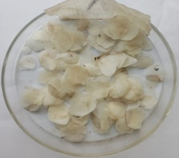
Plate 1. Cleaned Fish Scale
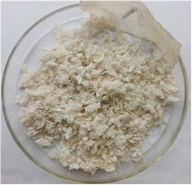
Plate 2. Ground Fish Scale
giving a total number of thirty (30) runs (Table 1). For the demineralization, thirty samples (30), each weighing 50 g, were taken from the ground fish scales and placed in separate conical flasks. Hydrochloric acid solutions with concentrations ranging from 0.5 to 6.5 M were prepared and added to the fish scales at a ratio of 1:10 w/v. The mixtures were gently stirred, and the demineralization process was allowed to proceed for different durations ranging from 12 to 48 hours. After the specified time, the demineralized fish scales were separated from the acid solution by filtration. To ensure the removal of any residual acid, the demineralized fish scales were rinsed with deionized water until the pH of the reached 7.00.
The demineralized fish scales were transferred to clean conical flasks. Sodium hydroxide solutions with concentrations ranging from 0.5 to 2.5 M were prepared and added to the fish scales at a solute-to-solvent ratio of 1:10 w/v. The mixtures were allowed to react for different durations ranging from 0.5 to 3.5 hours. After the specified time, the mixtures were filtered to achieve a filtrate pH of 7.00. The residue left after filtration was weighed to determine the yield of the deproteinization process. For the optimisation of the process, the sample with the maximum yield was reproduced using 1000g of the fish scale.
Experimental design and statistical analysis
The traditional approach for optimizing a multi-factorial system is to handle one variable at a time. However, this method is time-consuming, inefficient in terms of cost, and fails to uncover the interactive and quadratic effects of the factors. To address these limitations, Central Composite Design (CCD) of Response Surface Methodology (RSM) was chosen for the statistical optimization of chitin extraction from tilapia fish scale waste. Four experimental factors, including acid concentration, demineralization time, alkali concentration and deproteinization time (X1, X2, X3 and X4) were used for chitin production (Table 2). Each numeric factor is set to 5 levels: plus, and minus alpha (axial points), plus and minus 1 (factorial points) and the centre point. A quadratic regression model was employed to predict the response variable and fit the experimental data. The second-order polynomial equation was utilized for this purpose.
Determination and confirmation of optimal conditions
The optimal conditions were determined through the analysis of response surface plots and the composite desirability function. The objective was to achieve the highest yield % (Y) for chitin.
Table 1. Experimental Design for Chitin Production
| Factor 1 | Factor 2 | Factor 3 | Factor 4 | ||
| Std | Run | X1:HCl Conce-ntration | X2: Time of Demine-ralization | X3: NaOH Concent-ration | X4: Time of Deprotei-nization |
| (mol/dm3) | (hr) | (mol/dm3) | (hr) | ||
| 20 | 1 | 3.5 | 48 | 1.5 | 3.5 |
| 25 | 2 | 3.5 | 24 | 1.5 | 3.5 |
| 1 | 3 | 2 | 12 | 1 | 2 |
| 29 | 4 | 3.5 | 24 | 1.5 | 3.5 |
| 22 | 5 | 3.5 | 24 | 2.5 | 3.5 |
| 26 | 6 | 3.5 | 24 | 1.5 | 3.5 |
| 6 | 7 | 5 | 12 | 2 | 2 |
| 3 | 8 | 2 | 36 | 1 | 2 |
| 5 | 9 | 2 | 12 | 2 | 2 |
| 28 | 10 | 3.5 | 24 | 1.5 | 3.5 |
| 14 | 11 | 5 | 12 | 2 | 5 |
| 7 | 12 | 2 | 36 | 2 | 2 |
| 16 | 13 | 5 | 36 | 2 | 5 |
| 4 | 14 | 5 | 36 | 1 | 2 |
| 12 | 15 | 5 | 36 | 1 | 5 |
| 8 | 16 | 5 | 36 | 2 | 2 |
| 13 | 17 | 2 | 12 | 2 | 5 |
| 21 | 18 | 3.5 | 24 | 0.5 | 3.5 |
| 23 | 19 | 3.5 | 24 | 1.5 | 0.5 |
| 10 | 20 | 5 | 12 | 1 | 5 |
| 11 | 21 | 2 | 36 | 1 | 5 |
| 27 | 22 | 3.5 | 24 | 1.5 | 3.5 |
| 17 | 23 | 0.5 | 24 | 1.5 | 3.5 |
| 9 | 24 | 2 | 12 | 1 | 5 |
| 19 | 25 | 3.5 | 0 | 1.5 | 3.5 |
| 30 | 26 | 3.5 | 24 | 1.5 | 3.5 |
| 15 | 27 | 2 | 36 | 2 | 5 |
| 18 | 28 | 6.5 | 24 | 1.5 | 3.5 |
| 24 | 29 | 3.5 | 24 | 1.5 | 6.5 |
| 2 | 30 | 5 | 12 | 1 | 2 |
Table 2. Factorial Design for Chitin Production
| Name | Units | Low | High | -alpha | +alpha | |
| X1 | HCl Concent-ration | mol/dm3 | 2 | 5 | 0.5 | 6.5 |
| X2 | Time of Demine-ralization | hr | 12 | 36 | 0 | 48 |
| X3 | NaOH Concentration | mol/dm3 | 1 | 2 | 0.5 | 2.5 |
| X4 | Time of Deproteinization | hr | 2 | 5 | 0.5 | 6.5 |
To verify the optimized conditions, the experiments were repeated using the recommended RSM-based optimal conditions on Design- Expert 13 software. The experimental results were then compared with the predicted values. Additionally, the optimized response quadratic models were analytically confirmed by calculating the first derivatives of the mathematical functions that describe the response surface and equating them to zero.
Characterization of samples
Moisture content was assessed using the gravimetric method that involved drying the sample until a constant weight was achieved and measuring the weight of the sample before and after drying. The moisture content was then calculated using Equation 1:
Moisture Content = \( \frac{\text{wet sample (g)} – \text{dry sample (g)}}{\text{wet sample (g)}} \times 100 \) (1)
The chitin yield was calculated using Equation 2 in which \( Y = \text{yield}, M_1 = \text{mass of sample before the extraction}, M_2 = \text{mass of sample after the extraction}. \)
\( Y = \frac{M_2}{M_1} \times 100 \) (2)
The bulk density (ρb) of the experimentally produced sample was determined by measuring the volume of distilled water displaced by a known mass of each sample. After drying the samples at 105°C, a measured weight of the adsorbent was placed into a 10 ml graduated cylinder. The cylinder was gently tapped on the laboratory bench top until no further reduction in the sample level was observed. The bulk density (ρb) was calculated using the Equation 5 in which m = mass of sample, v = volume displaced.
\(\rho_b = \frac{m}{v} \qquad (3)\)
The pH of the sample was measured by weighing 1 g portion of the dried sample into a 100 mL beaker. Subsequently, 30 mL of distilled water was added to the beaker. The mixture was then heated to boiling and allowed to digest for 10 minutes. Afterward, the solution was filtered while still hot. The filtrate was cooled to room temperature, and the pH of the solution was determined using a pH meter.
The ash content of each sample was determined by placing 1 g of the sample into previously weighed crucible. The crucible and its contents were then placed in an electric oven at 110°C for about 4 hours. The sample was heated in an electric muffle furnace at 600 °C for 2 hours. The crucible was allowed to cool in desiccator for 30 minutes. The heating and cooling process was then repeated until the difference between two consecutive weights was less than 1 mg and a white ash is obtained. The % ash was determined using Equation 4 in which W1 = weight of residue (g), W = weight of the sample taken for the test (g), X = percentage of moisture content present in the sample taken for the test.
\(\% \text{ Ash Content} = \frac{W_1}{W \left(\frac{100 – X}{100}\right)} \times 100 \qquad (4)\)
To determine the functional groups of the samples, FTIR analysis was performed. A few crystals were mixed with potassium bromide (KBr) and pulverized in an agate mortar to form a homogenous powder from the appropriate pellet was prepared under a pressure of 7 tons. All spectra were recorded from 4000 to 400 cm-1 using the Pelkin Elmer 3000 MX spectrometer. Scans were 32 per spectrum with a resolution of 4 cm-1. The IR spectra were analysed using the spectroscopic software Win-IR Pro Version 3.0 with a peak sensitivity of 2cm1. The graph of percentage transmittance against wavelength was obtained and the peak points were noted for determining the functional groups of the samples.
Scanning Electron Microscope (SEM) was used to obtain valuable information about the sample morphological structure and characteristics quantitative X-rays microanalysis. Samples used for SEM analysis were appropriately sized to fit in the specimen chamber and were mounted rigidly on a specimen holder known as a specimen stub. To enhance the electrical conductivity of the samples, they were coated with a layer of platinum. The prepared sample was places in a relatively high-pressure chamber, where the working distance between the sample and the electron optical column is short. The electron optical column was differentially pumped to maintain an adequately low vacuum level at the electron gun. This high-pressure region surrounding the sample in the Environmental SEM (ESEM) neutralizes charge and enhances the amplification of the secondary electron signal.
RESULTS AND DISCUSSION
Statistical Analysis and Optimization
The Central Composite Design (CCD) in Response surface methodology gave the combination of parameters for the yield of chitin from tilapia fish scale waste. The yield of each run is presented in Table 3. The results shows that the yield of the chitin falls in the range of 0 and 22%. The CCD gave different sources for regression equation for the process. A quadratic regression model equation was suggested for predicting the optimal point of chitin extraction yield from the tilapia fish scale. The sources are presented in Table 4 and the suggested regression equation is given in Equation 1. The equation, expressed in terms of actual factors, enables us to make predictions regarding the response based on specific levels of each factor. It is essential to specify these levels in the original units associated with each factor to ensure accurate predictions. However, it is important to note that this equation should not be utilized to determine the relative impact of each factor. The coefficients in the equation are scaled to account for the units of each factor, and the intercept is not situated at the centre of the design. As a result, comparing the coefficients directly may lead to incorrect conclusions regarding the relative importance or influence of each factor on the response. Therefore, caution should be exercised when interpreting the coefficients in terms of their magnitudes. The optimum production conditions being 1M HCl, 12 hours demineralization, 1M NaOH and 2 hours deproteinization on maximizing the yield of Chitin and minimizing other parameters giving a yield of 34%.
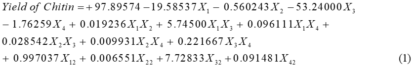
Table 3. Yield of Chitin from Experimental runs
| Run | Factor 1 | Factor 2 | Factor 3 | Factor 4 | Response |
| X1: HCl Concen-tration | X2: Time of Deminer-alization | X3: NaOH Concentra-tion | X4: Time of Deproteiniz-ation | Y: Yield of Chitin | |
| 1 | 3.5 | 48 | 1.5 | 3.5 | 0.1 |
| 2 | 3.5 | 24 | 1.5 | 3.5 | 0.35 |
| 3 | 2 | 12 | 1 | 2 | 22 |
| 4 | 3.5 | 24 | 1.5 | 3.5 | 0.34 |
| 5 | 3.5 | 24 | 2.5 | 3.5 | 0.01 |
| 6 | 3.5 | 24 | 1.5 | 3.5 | 0.35 |
| 7 | 5 | 12 | 2 | 2 | 1.4 |
| 8 | 2 | 36 | 1 | 2 | 18.5 |
| 9 | 2 | 12 | 2 | 2 | 3.5 |
| 10 | 3.5 | 24 | 1.5 | 3.5 | 0.35 |
| 11 | 5 | 12 | 2 | 5 | 1.1 |
| 12 | 2 | 36 | 2 | 2 | 1.2 |
| 13 | 5 | 36 | 2 | 5 | 0.5 |
| 14 | 5 | 36 | 1 | 2 | 0.5 |
| 15 | 5 | 36 | 1 | 5 | 0.3 |
| 16 | 5 | 36 | 2 | 2 | 0.14 |
| 17 | 2 | 12 | 2 | 5 | 2.5 |
| 18 | 3.5 | 24 | 0.5 | 3.5 | 15.5 |
| 19 | 3.5 | 24 | 1.5 | 0.5 | 1.5 |
| 20 | 5 | 12 | 1 | 5 | 1.3 |
| 21 | 2 | 36 | 1 | 5 | 17.5 |
| 22 | 3.5 | 24 | 1.5 | 3.5 | 0.35 |
| 23 | 0.5 | 24 | 1.5 | 3.5 | 18 |
| 24 | 2 | 12 | 1 | 5 | 20 |
| 25 | 3.5 | 0 | 1.5 | 3.5 | 7.5 |
| 26 | 3.5 | 24 | 1.5 | 3.5 | 0.35 |
| 27 | 2 | 36 | 2 | 5 | 0.9 |
| 28 | 6.5 | 24 | 1.5 | 3.5 | 0 |
| 29 | 3.5 | 24 | 1.5 | 6.5 | 0.2 |
| 30 | 5 | 12 | 1 | 2 | 2 |
Table 4. Fit Summary of the Yield of Chitin
| Source | Sequential p-value | Lack of Fit
p-value |
Adjusted R² | Predicted R² | |
| Linear | < 0.0001 | < 0.0001 | 0.6034 | 0.5004 | |
| 2FI | 0.0077 | < 0.0001 | 0.7748 | 0.7354 | |
| Quadratic | < 0.0001 | < 0.0001 | 0.9888 | 0.9666 | Suggested |
| Cubic | 0.0194 | < 0.0001 | 0.9966 | 0.8834 | Aliased |
As shown in Table 4, the results indicate a strong level of agreement between the Predicted R² (0.9666) and the Adjusted R² (0.9888), with the difference between them being less than 0.2. This suggests that the model’s predictions are highly consistent and reliable. Furthermore, the Adeq Precision ratio, which measures the signal to noise ratio, is exceptionally high at 40.283 (Table 5). A ratio above 4 is generally considered desirable, indicating a strong signal. In this case, the significantly higher ratio indicates that the signal in the model is much stronger than the noise. Consequently, the model proves to be well-suited for navigating the design space, providing valuable insights and reliable predictions. Table 5 and Figure 1 shows that the difference between the predicted and actual values are close and are acceptable. The significant
Table 5. Fit Statistics and Comparison of Actual Yield and Predicted Yield
| Std. Dev. | 0.7735 | R² | 0.9942 |
| Mean | 4.61 | Adjusted R² | 0.9888 |
| C.V. % | 16.79 | Predicted R² | 0.9666 |
| Adeq Precision | 40.283 | ||
| Run | Actual Value | Predicted Value | Residual |
| 1 | 0.1 | 1.7 | -1.6 |
| 2 | 0.35 | 0.3483 | 0.0017 |
| 3 | 22 | 21.62 | 0.3771 |
| 4 | 0.34 | 0.3483 | -0.0083 |
| 5 | 0.01 | -0.41 | 0.42 |
| 6 | 0.35 | 0.3483 | 0.0017 |
| 7 | 1.4 | 1.76 | -0.3646 |
| 8 | 18.5 | 17.81 | 0.6912 |
| 9 | 3.5 | 3.84 | -0.3437 |
| 10 | 0.35 | 0.3483 | 0.0017 |
| 11 | 1.1 | 1.53 | -0.4271 |
| 12 | 1.2 | 0.7146 | 0.4854 |
| 13 | 0.5 | 0.4979 | 0.0021 |
| 14 | 0.5 | -0.1204 | 0.6204 |
| 15 | 0.3 | -0.3079 | 0.6079 |
| 16 | 0.14 | 0.0204 | 0.1196 |
| 17 | 2.5 | 2.74 | -0.2412 |
| 18 | 15.5 | 16.56 | -1.06 |
| 19 | 1.5 | 1.82 | -0.3167 |
| 20 | 1.3 | 1.41 | -0.1062 |
| 21 | 17.5 | 16.76 | 0.7437 |
| 22 | 0.35 | 0.3483 | 0.0017 |
| 23 | 18 | 18.89 | -0.8933 |
| 24 | 20 | 19.86 | 0.1446 |
| 25 | 7.5 | 6.54 | 0.9567 |
| 26 | 0.35 | 0.3483 | 0.0017 |
| 27 | 0.9 | 0.3271 | 0.5729 |
| 28 | 0 | -0.25 | 0.25 |
| 29 | 0.2 | 0.5267 | -0.3267 |
| 30 | 2 | 2.31 | -0.3087 |
Model F-value of 183.88 indicates that the model is of importance (Table 6). The probability of such a large F-value occurring purely by chance is only 0.01%. Model terms with p-values below 0.0500 are considered significant, suggesting their importance in the model. In this case, the terms X1, X2, X3, X1X3, X12, X22, and X32 are all significant. Conversely, p-values exceeding 0.1000 indicate that the model terms are not significant. If there are numerous insignificant model terms (excluding those necessary for hierarchical support), reducing the model may enhance its performance (Table 6). Figures 2
and 3 shows surface and contour plots, respectively, for the correlation between the response (Yield) and the independent variables.
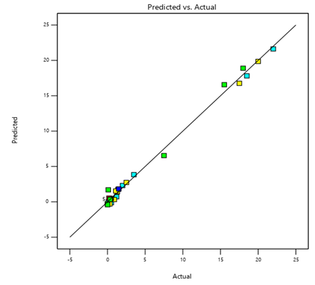
Figure: 1. Plot of Predicted Value vs Actual Value
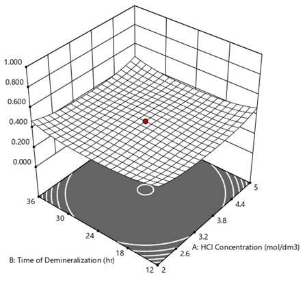
Figure 2. Surface Plot for Yield and the Independent variables
Table 6. Analysis of Variance for the Quadratic Mode
| Source | Sum of Squares | Mean Square | F-value | p-value | |
| Model | 1540.26 | 110.02 | 183.88 | < 0.0001 | Signifi-cant |
| X1-HCl Concentration | 549.7 | 549.7 | 918.73 | < 0.0001 | |
| X2-Deminera-lization Time | 35.19 | 35.19 | 58.81 | < 0.0001 | |
| X3-NaOH Concentr-ation | 432.14 | 432.14 | 722.25 | < 0.0001 | |
| X4-Deprotein-ization Time | 2.5 | 2.5 | 4.17 | 0.0591 | |
| X1X2 | 1.92 | 1.92 | 3.21 | 0.0936 | |
| X1X3 | 297.05 | 297.05 | 496.46 | < 0.0001 | |
| X1X4 | 0.7482 | 0.7482 | 1.25 | 0.281 | |
| X2X3 | 0.4692 | 0.4692 | 0.7842 | 0.3898 | |
| X2X4 | 0.5112 | 0.5112 | 0.8544 | 0.3699 | |
| X3X4 | 0.4422 | 0.4422 | 0.7391 | 0.4035 | |
| X12 | 138.04 | 138.04 | 230.7 | < 0.0001 | |
| X22 | 24.41 | 24.41 | 40.79 | < 0.0001 | |
| X32 | 102.39 | 102.39 | 171.13 | < 0.0001 | |
| X42 | 1.16 | 1.16 | 1.94 | 0.1837 | |
| Residual | 8.97 | 0.5983 | |||
| Lack of Fit | 8.97 | 0.8975 | 53849 | < 0.0001 | Signifi-cant |
| Pure Error | 0.0001 | 0 | |||
| Cor Total | 1549.24 |
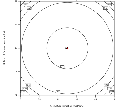
Figure 3. Contour Plot for Yield and the Independent Variables
This shows the predictability of the response in the absence of real-time values. The independent variables are inversely proportional to the response.
Proximate Properties
Table 7 shows the physiochemical properties of the extracted chitin with the pH value being almost neutral indicating that have values to show the quality of the product and being neither acidic nor alkaline. The bulk density of the sample is 0.15g/ml which is relatively low. This indicates that the sample is porous and loosely pack. This can be advantageous in applications such as pharmaceutical industry for drug delivery.
Table 7. Proximate Properties
| Bulk Density | 0.15g/ml |
| Moisture content | 9.6% |
| Ash Content | 3.1% |
| pH |
SEM Result Analysis
The SEM analysis of the chitin obtained from tilapia fish scale waste provides valuable insights into the morphological characteristics of the extracted material (Figure 4). The SEM images reveal the surface and structural features of the chitin, allowing for a detailed examination of its physical properties. The SEM images of the chitin show a fibrous and porous structure. The fibres appear to be elongated and intertwined, forming a network-like arrangement.
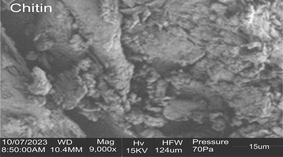
Figure 4. SEM image of the produced Chitin
The porous nature of the chitin is evident from the presence of irregularly shaped voids and channels throughout the material. These pores contribute to the overall surface area and porosity of the chitin, which can have implications for its potential applications. The observed fibrous structure of the chitin is desirable, as it provides mechanical strength and flexibility to the material. The interconnected fibres offer a large surface area for interactions with other substances, making the chitin suitable for various functional applications. The fibrous morphology also suggests that the extraction process effectively separates the chitin from other components of the fish scales, such as proteins and minerals. The porosity of the chitin is advantageous for applications that require absorption, adsorption, or filtration capabilities. The presence of pores can facilitate the uptake and release of molecules, making chitin a promising material for drug delivery systems, water treatment, and wound healing applications. The size and distribution of the pores can further influence the material behaviour and performance in specific applications. It is important to note that the observed morphology of the chitin may vary depending on the extraction method employed and the specific characteristics of the tilapia fish scales used. Different extraction techniques and conditions can yield chitin with varying degrees of porosity, fibber arrangement, and surface characteristics.
FTIR Result Analysis
FTIR analysis of chitin extracted from tilapia fish scales provides indicates the molecular structure and composition of the extracted chitin. The FTIR spectrum of chitin extracted from tilapia fish scales exhibits characteristic absorption bands associated with chitin unique functional groups (Figure 5). The presence of a strong band at approximately 1652.21 cm-1 corresponds to the amide I band, indicating the presence of C= O stretching vibrations. Another strong band observed around 1543 cm-1 corresponds to the amide II band, indicating N-H bending and C-N stretching vibrations. These bands confirm the presence of chitin in the extracted sample. However, for α-chitin, the amide I band split into two distinct components, appearing at 1660 and 1630 cm-1 attributed to factors such as hydrogen bonding within the amide structure. Conversely, in β-chitin, the amide I band is singular, occurring solely at 1630 cm-1. Notably, both chitin allomorphs display the presence of the amide II band at single band. This observation suggests that the type of chitin produced in this study corresponds to β-chitin, as indicated by the singular amide I band at 1652 cm-1. By comparing the obtained spectrum with reference spectra of chitin, it identifies purities and other compounds that may be present in the sample.

Figure 5. Absorption Spectra of Produced Chitin
Absence CH2 wagging (Amine III) component around the peaks of 1318 corresponding to protein residues, lipids, or other organic compounds in the FTIR spectrum would suggest a high-purity chitin sample. The positions and intensities of the absorption bands in the FTIR spectrum tells the arrangement of chitin chains, intra- and intermolecular hydrogen bonding, and other structural characteristics. The degree of crystallinity is estimated by analysing the intensity of the band at around 871 cm^-1, corresponding to the C-O-C stretching vibration. A high intensity indicates a more crystalline structure.
The absorption spectra of chitin typically exhibit several characteristic peaks associated with its functional groups. While the exact peak numbers vary slightly with some commercial chitin of alpha amorphous which could be attributed to factors such as sample preparation and instrument settings and variation the amorphous. Some common absorption peak numbers observed in the FTIR spectra of chitin are given in Table 8 for comparison. For α-chitin, the amide I band is split into two components at 1660 and 1630 cm -1 (due to the influence of hydrogen bonding or the presence of an enol form of the amide, whereas for β-chitin it is at 1630 cm -1. The amide II band is observed in both chitin allomorphs: at 1558 cm -1 for α-chitin and 1562 cm -1 for β-chitin.
Table 8. Comparison of Absorption Regions and Functional Groups of the Chitin
| Functional group assignment | Commercial Chitin region (cm-1) [16] | Sigma Aldrich Chitin region (cm-1) [5] | Experimental Chitin region (cm-1) [this study] |
| O-H stretch (water) | 3700-3200 | 3456 | 3391 |
| N-H stretch (amine) | 3100-3500 | – | – |
| C-H symmetrical stretch (aliphatic) | 2937-2867 | 2880 | 2925-2859 |
| C=O stretch (amide I) | 1654 – 1620 | 1662-1625 | 1652 |
| N-H bend/C-N stretch (amide II) | 1553 | 1560 | 1543 |
| CH2 ending/CH3 deformations II) | 1430 | 1433 | 1451 |
| CH bends CH3 symmetrical | 1376 | 1382 | – |
| CH2wagging (Amine III), Protein component | 1318 | 1313 | – |
| Asymmetric bridge oxygen stretching | 1155 | 1158 | 1165 |
| C–O asymmetric stretch in phase ring | 1024 | 1027 | 1025 |
| CH3 wagging | 952 | – | – |
| CH ring stretching (Saccharide rings) | 896 | – | 871 |
Comparison analysis with other chitin extraction methods
While this study focuses on optimizing chitin extraction from tilapia fish scales, it is essential to compare its efficiency with conventional extraction methods such as enzymatic hydrolysis, which is a biological method. The traditional chemical method used in this study involved acid demineralization and alkali deproteinization. The chemicals are widely employed due to their simplicity and effectiveness in getting the targeted chitin [3]. However, biological method is a clean process but the efficiency is lower in comparison to the chemical processes as around 5%–10% protein is still remained and associated with the isolated chitin. Also, various factors are needed to be considered and controlled in the biological methods. including initial pH, type of substrate, concentrate of substrate, fermentation time, and by-products, which could lead to complicated product and error [4]. The time for the chitin extraction in this study was 14 hours which is acceptable for batch process. whereas the biological methods usually take about 24-72 hours.
Scalability and economic feasibility for industrial applications
The feasibility of large-scale chitin production depends on economic and operational factors, including reagent costs, process efficiency, and environmental impact. The optimized conditions in this study—1M HCl for 12 hours demineralization and 1M NaOH for 2 hours deproteinization—suggest a relatively moderate consumption of chemicals, making it more cost-effective than processes requiring high acid or alkali concentrations. However, industrial-scale production must consider waste treatment, as strong acid and alkali usage can lead to significant effluent management costs [9]. In contrast, biological method offers a more sustainable alternative but may require longer processing times and higher operational costs due to enzyme procurement. Thus, the optimized method presented here balances cost and efficiency, but future research should explore strategies, for minimizing chemical usage and enhancing recycling to improve environmental sustainability.
CONCLUSION
The extraction of chitin from tilapia fish scales was investigated to determine the optimal operating conditions. The optimal product was achieved at 1M HCl for 12 hours demineralization and 1M NaOH at 2 hours deproteinization to produce the Chitin. The agreement between the Predicted R² (0.9666) and the Adjusted R² (0.9888) from the statistical analysis of the extraction process suggests high consistency and reliability of the model predictions. The distinctive peaks observed in the FTIR spectra shows a single band for amide I at 1652 cm^-1 (amide I) representing C=O stretching vibrations, and another at 1543 cm^-1 (amide II) indicating N-H bending and C-N stretching vibrations, confirming the presence of β-chitin. Additionally, the SEM analysis revealed the morphological features of the extracted chitin, showcasing its fibrous and porous nature. The SEM images provided visual evidence of the successful isolation and extraction of chitin from the tilapia fish scales. Furthermore, the properties of the extracted chitin were investigated, revealing important characteristics such as moisture content, ash content, bulk density and pH being 9.6%, 3.1%, 0.15 g/ml and 7.2 respectively These properties contribute to the overall functionality and potential applications of chitin in various industries, including pharmaceuticals, agriculture, and food.
ACKNOWLEDGMENT
The authors gratefully acknowledge the support from Lagos State University during the research work
REFERENCES
- Abidin, N.A., Kormin, F., Abidin, N. A., Anuar, N.A.F.M.A., Bakar, M.F.A. (2020). The Potential of Insects as Alternative Sources of Chitin: An overview on the chemical method of extraction from various Sources: A Review. International Journal of Molecular Science .21, 4978; doi:10.3390/ijms21144978.
- Lizundi, E., Nguyen, T.-D., Winnick, R. J., & MacLachlan, M. (2021). Biomimetic photonic materials derived from chitin and chitosan. J. Mate. Chem. 3, 796–817. doi:10.1039/D0TC05381C.
- Yan, N., & Chen, X. (2015). Sustainability: don’t waste seafood waste. Nature 524, 155–157.
- Yadav, M., Goswami, P., Paritosh, K., Kumar, M., Pareek, N., & Vivekanand, V. (2019). Seafood waste:a source for preparation of commercially employable chitin/chitosan materials. Bioresour. Bioprocess , 6, 8. https://doi.org/10.1186/s40643-019-0243-y
- Olafadehan, O. A., Abhulimen, K. E., Adeleke, A. I., Njoku, C. V., & Amoo, K. O. (2019). Production and characterization of derived composite biosorbents from animal bone. African Journal of Pure and Applied Chemistry 13(2), 12–26. https://doi.org/10.5897/ajpac2018.0765.
- Sanjanwala, D., Londhe, V., Trivedi, R., Bonde, S. Sawarkar, S., Kale, V., Patravale, V. (2022). “Polysaccharide-based hydrogels for drug delivery and wound management: a review”. Expert Opinion on Drug Delivery. 19(12): 1664–1695. doi:10.1080/17425247.2022.2152791
- Morin-Crini, N., Lichtfouse, E., Torri, G., Crini, G., (2019). Applications of chitosan in food, pharmaceuticals, medicine, cosmetics, agriculture, textiles, pulp and paper, biotechnology, and environmental chemistry. Environmental Chemistry Letters. 17 (4): 1667–1692. doi:1007/s10311-019-00904-x.
- El Hadrami, A; Adam, L. R.; El Hadrami, I; Daayf, F (2010). “Chitosan in plant protection”. Marine Drugs. 8(4): 968–987.
- Debode, J., De-Tender, C., Soltaninejad, S., Van-Malderghem, C., Haegeman, A., Van der-Linden, I., Cottyn, B., Heyndrickx, M., Maes, M. (2016). “Chitin mixed in potting soil alters lettuce growth, the survival of zoonotic bacteria on the leaves and associated rhizosphere microbiology”. Frontiers in Microbiology. 7: 565. https://doi:10.3389/fmicb.2016.00565
- Tzoumaki, M. V., Moschakis, T., Kiosseoglou, V., Biliaderis, C. G. (2011). Oil-in-water emulsions stabilized by chitin nanocrystal particles”. Food Hydrocolloids 25, 1521–1529. doi:1016/j.foodhyd.2011.02.008
- Oluwatoosin, B. A., Glenn, A. B., Zhifei, Z., Kingsley, C. D., Yue, L., Simon, C. G., & Lars, E. H. (2021). Composites & nanocomposites :Biomacromolecules in recent phosphate-shelled brachiopods: identification and characterization of chitin matrix. Journal of Material scienc 56:19884–19898. https://doi.org/10.1007/s10853-021-06487-9.
- Lee, T., Mohd Pu’ad, N. A., Alipal, J., Muhamad, M. S., Basri, H., Idris, M. I., & Abdullah, H. (2022). Tilapia wastes to valuable materials: A brief review of biomedical, wastewater treatment, and biofuel applications. Materials Today: Proceedings (1389-1395. https://doi.org/10.1016/j.matpr.2022.03.174
- Ángela, G. G., Marnie, C. Q., & Hans, T. C. (2019). Extraction and characterization of chitin scales from red tilapia (oreochromis sp.) from Huila, Colombia by chemical methods . Revista Ingenierías Universidad de Medellín 18, https://doi.org/10.22395/rium.v18n34a5
- Marian, A.-N., Asare, B. D., Gabriel, A. A., & Junias, A.-G. (2022). Evaluation of Scales of Tilapia Sp. and Sciaenops ocellatus as low cost and green adsorbent for fluoride removal from water. Frontiers in Chemistry 10.
- Lee, T., Mohd Pu’ad, N. A., Alipal, J., Muhamad, M. S., Basri, H., Idris, M. I., & Abdullah, H. (2022). Tilapia wastes to valuable materials: A brief review of biomedical, wastewater treatment, and biofuel applications. Materials Today: Proceedings, 1389-1395 https://doi.org/10.1016/j.matpr.2022.03.174
- Kaya, M., Lelesius, E., Nagrockaite, R., Sargin, I., Arslan, G., Mol, A., (2015). Differentiations of chitin content and surface morphologies of chitins extracted from male and female grasshopper species. PLoS ONE 10 (1): e0115531. Doi.10.1371/journal.pone.0115531