
Theoretical and Simulation Finite Element Modal Analysis of Rotating Cantilever Beam
- Abonyi Sylvester Emeka
- Ilechukwu Anthonia Ekene
- Omenyi Sam
- Okafor Anthony Amaechi
- Odeh Calistus Princewill
- 291-306
- Mar 21, 2024
- Architecture
Theoretical and Simulation Finite Element Modal Analysis of Rotating Cantilever Beam
1Ilechukwu Anthonia Ekene, 1Omenyi Sam, 3Abonyi Sylvester Emeka*, 4Okafor Anthony Amaechi, 5Odeh Calistus Princewill
1Mechanical Engineering Department, Nnamdi Azikiwe University Awka, Nigeria;
2Electrical Engineering Department, Nnamdi Azikiwe University Awka, Nigeria
*Corresponding Author
DOI: https://doi.org/10.51584/IJRIAS.2024.90225
Received: 15 January 2024; Accepted: 12 February 2024; Published: 21 March 2024
ABSTRACT
The finite element method is used to carry out modal analysis of rotating cantilever beam. The virtual work method is then used to derive the stiffness matrix of a rotating beam element. The stiffness matrix of a rotating beam element is simply seen to be sum of the stiffness matrix of the non-rotating beam and an incremental stiffness matrix induced by rotation. This work presents a novel generalized incremental stiffness matrix that takes care of any element at any distance from the rotation axis. The established rotational stiffness matrix is then used together with consistent mass matrix (not affected by rotation) to carry out modal analysis of rotating cantilever beam. Theoretical computations were validated by simulations from ANSYS. It is seen that the contribution to modal frequencies and shapes of the blade of rotation via incremental stiffness matrix is very marginal at low rotational speeds. For example it is seen for a numerical case study that five-element model computes slight increase in fundamental natural frequency due to rotation relative to that of the non-rotating blade as 0.000195% for rotational speed of 300rpm. It is also seen that ten times increase in speed leads to about hundred times increase in rotational contribution meaning that it becomes more imperative to model rotation as speed of the blade increases. Points are also made regarding application to avoiding resonance of rotating cantilever beam.
Keyword: cantilever beam, helicopter blades, modal analysis, vibration
INTRODUCTION
Rotating beams are of two types of application. The first type is shaft rotating about its longitudinal axis [1-4] which has application in power transmission. The second type involves a blade rotating about its normal axis [5-10] which has application aerospace. The second type is of interest in this work thus given a more detailed review. At the beginning of the last century Southwell and Gough [5] pioneered research on modal analysis of rotating cantilever beams. Yntema [6] presented and demonstrated use of simplified procedures and charts for the rapid estimation of bending frequencies of rotating beams. In [9] warping inhibition and centrifugal force in addition to free vibration behaviour of rotating blades modelled as hollow boxed beams were considered. Huang et al. in the work [10] considered slender beam rotating at high angular velocity and proposed a method based on the power series solution to determine the modal frequencies of such system. A very popular application of the second type in aerospace industry is in modal analysis helicopter blades. Helicopters are of very popular use in civilian, executive and military transport. They are very convenient for transportation because of their capacity to hover and take off or land vertically. Vibrations stemming from the rotating blades are always a source of inconvenience for passengers in the cabin. Other major negative effects of these vibrations are degradation of structural integrity, reduction in component fatigue life, impairment of computerized control systems essential in navigation, and crash due to catastrophic failure of any of the blades. A basic reason for catastrophic failure of any of the blades is excitation that occurs at any of the blade natural frequencies due to excessive resonant vibrations. Blade loads are comprised of both aerodynamic and inertial contributions at harmonics of the rotor speed, The sectional inertial and aerodynamic blade loads can be integrated along the blade length to obtain the blade root loads, also at harmonics of .These blade root loads from every blade are summed at the rotor hub to yield periodic hub loads which could be very catastrophic at resonant conditions. Over the years performance of helicopters has been optimized. A passive strategy that has been employed to minimize vibrations is blade design optimization. Blade design optimization includes proactive measures in rotor blade structural and aerodynamic properties leading to reduced overall vibration [12, 13]. The classical design parameters always mentioned are rotor tip sweep, taper, non-structural mass distribution, structural stiffness, elastic tailoring and spar cross-sectional geometry [14]. The interest in this work is to use the method of finite element in forestalling resonant vibration in the flap-wise direction of rotating cantilever beam by investigating the effect of rotation on natural response to initial conditions. Theoretical computation will be validated by additional results from ANSYS simulation. This is geared towards excessive resonant response to rotational harmonic forces. The blades are also subjected to lag and torsion vibrations in addition to flap vibrations as shown in figure 1. It is also noteworthy the three kinds of rigid motion of a helicopter; yaw, roll and pitch as also shown in figure1. The presentations in this work will subsequently be applied to study of flap-wise vibration of the blades considering the aforementioned design parameters. The flap-wise vibration is normally studied because structural weakness of blade in this direction that exposes it to sudden failure.
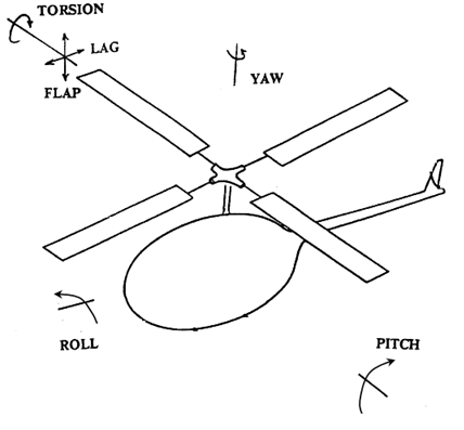
Fig.1. A typical helicopter showing the three kinds of rigid motion; yaw, roll and pitch and blade vibrations; Flap, Lag and torsion. Adapted from [11].
- General beam Finite element modelling
The matrix model for transient response of a non-rotating beam finite element shown in fig. 2 is
![]() (1)
(1)
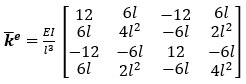
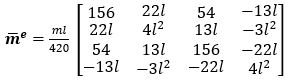
The stiffness matrix k ̅e and the consistent mass matrix ![]() are given by [15], [16]
are given by [15], [16]
 (2)
(2)
 (3)
(3)
Where E, I, m and l are the young modulus, area moment of inertia about the neutral axis, mass per unit length and length of the beam respectively.
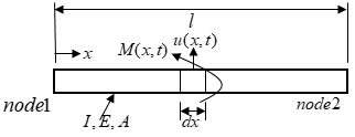
Fig. 2. A finite non-rotating beam element
Suppose the beam is then subjected to some form of time-invariant distributed force per unit length of the element f(x), the nodes of the element will experience nodal force vector fe that corresponds to the distributed force f(x) such that equation (1) becomes
![]() (4)
(4)
The general form for fe when f(x) is proportional to the local coordinate x is
![]() (5)
(5)
Where k ̅e,in is the incremental stiffness due to the distributed force f(x). Inserting “(4)” in “(5)” and re-arranging gives the transient response
![]() (6)
(6)
The principle of virtual work is used in determining the nodal force vector fe to have the form k ̅e,inu.
- Incremental stiffness matrix of the rotating beam element
The rigour associated with handling the rotating beam element revolves around derivation of the incremental stiffness k ̅e,in. Fig. 3 depicts a beam element rotating at angular speed Ω [rpm].
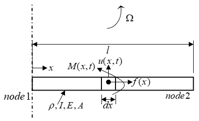
Fig. 3. A finite rotating beam element
A differential element dx of the beam is then subjected to the centrifugal force ![]() . This means that the distributed force f(x) reads
. This means that the distributed force f(x) reads
![]() (7)
(7)
The distributed force will do a virtual work given by
![]() (8)
(8)
The cumulative virtual work done by the element becomes
![]() (9)
(9)
The distributed deformation u(x) along the beam element is given by finite element formulation in terms of nodal displacements ui using the Hermite shape functions Ni(x) as
![]() (10)
(10)
Where
![]() (11)
(11)
![]() (12)
(12)
![]() (13)
(13)
![]() (14)
(14)
Inserting “(10)” into “(9)” and re-arranging gives
![]() (15)
(15)
The i th term of the nodal force vector fe becomes
![]() (16)
(16)
In view of “(16)” it is seen that the element ![]() of the incremental stiffness matrix is given generally by
of the incremental stiffness matrix is given generally by
![]() (17)
(17)
In light of “(7)”, “(17)” becomes
![]() (18)
(18)
Suppose a beam of length nl is regularly discretized into n elements and the eth element where e=1,2,3,…..n, is considered. The location of the differential element dx from rotational axis becomes rl+x where x is used as the local coordinate of the th element. “(7)” for centripetal force becomes ![]() which is then re-written as
which is then re-written as
![]() (19)
(19)
The element of incremental stiffness matrix given in “(18)” becomes
 (20)
(20)
“(20)” is the general equation for populating the incremental stiffness matrix k ̅e,in of the th rotating beam element about the rotational axis. It should be noted that “(18)” and “(20)” are identical for the first element. The first term of ‘(20)” is increment to ki,je,in as given in “(18)” for the first element due to displacement of the first local node from the rotational axis. The incremental stiffness matrix of a one-element beam resulting from use of “(18)” with notation ![]() is
is
 (21)
(21)
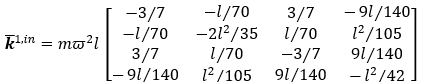
It must be noted that inserting e=1 in “(20)” gives same result as “(21)”. It must always be recalled that refers to length of beam element and not the length of the studied beam. With this in mind, a rotating beam of five elements each of length is then considered. The incremental stiffness matrix of the first element will have same form as “(21)”. For the second element, “(20)” is used with e=2 to give.
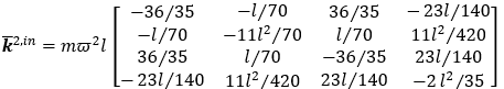 (22)
(22)
The incremental stiffness matrices of the third, fourth and fifth elements are derived using “(20)” with e=3,4 and 5 to give.
 (23)
(23)
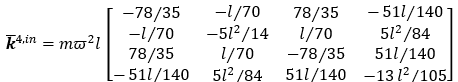 (24)
(24)
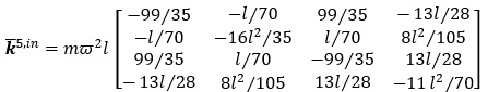 (25)
(25)
- Incremental global stiffness matrix of rotating beam
The rotating beam of length nl is regularly discretized into n elements. Since the beam is a cantilever the degree of freedom becomes 2n such that the representative global vector of nodal displacements becomes
![]() (26)
(26)
The nodal displacements of the eth element where e=2,3,…..n corresponds to the coordinates {U2e-3 U2e-2 U2e-1 U2e }T in the global vector U. This means that the second node of the (e-1)th and the first node of the eth element associate in the global matrix. This is the rule in assemblage of elements modelling the beam. The first node of the first element is fixed by boundary conditions imposed on cantilever beam such that the corresponding two degree of freedom coordinate becomes {U1 U2 }T. Modelling the blade with one beam element give the global incremental stiffness matrix
![]() (27)
(27)
Modelling the blade with three beam elements gives the global incremental stiffness matrix
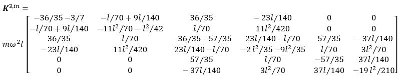 (28)
(28)
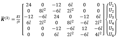
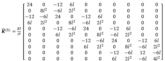
Modelling the blade with five beam elements gives the global incremental stiffness matrix
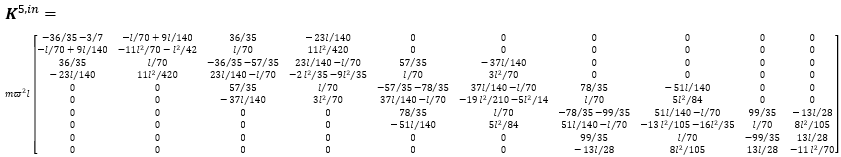 (29)
(29)
- The stiffness and mass matrices of non-rotating beam
The corresponding assembled stiffness matrices of the non-rotating mode of the beam are
![]() (30)
(30)
 (31)
(31)
 (32)
(32)
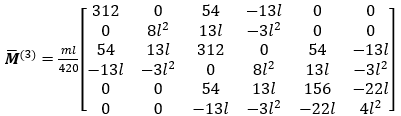
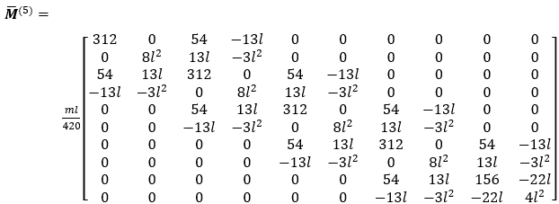
The corresponding assembled mass matrices of the non-rotating mode of the beam are
![]() (33)
(33)
 (34)
(34)
 (35)
(35)
- Numerical modal analysis and Discussions
The governing equation of transient response of the assembled model reads
![]() (36)
(36)
Where e is the number of elements of a chosen model. Modal analysis requires that the rotating structure is subjected to harmonic excitation. The resulting Eigen-value problem becomes
![]() (37)
(37)
For which ω is the circular frequency of the harmonic response. Post-multiplying with ![]() gives
gives
![]() (38)
(38)
It is seen from this form that ω2 is the eigen-value of the square symmetric matrix ![]() . The trivial solution of the homogenous “(37)” is of form U=0. The non-trivial solution of the homogenous “(37)” requires a null determinant;
. The trivial solution of the homogenous “(37)” is of form U=0. The non-trivial solution of the homogenous “(37)” requires a null determinant;
![]() (39)
(39)
Since the degree of freedom of the studied system is there will then eigen-values designated ω1, ω2…….. ω2n-1, and ω2n where the corresponding eigen-vectors satisfying “(37)” are designated U(1), U(2)……..U(2n-1) and U(2n).
A typical kinematic, dimensional and material specification for design of a real helicopter blade presented in [17] is adopted for numerical simulation. The helicopter blade is made of aluminium material, rotates at Ω=300 rpm and has the dimensions; 0.0254m (thickness) by 0.3048m (width) by 1.2192m (length). The relevant mechanical properties of pure aluminium are [18]; density ρ=2.7×10³ kgm-3 and young modulus E=70.5 GPa. The blade is recommended to be modelled with beam elements. The area moment of inertia for transverse vibration is given as ![]() where B is the width and thickness D is the thickness. The mass per unit length becomes ρBD=2.7×10^3×0.3048×0.0254=20.903184 kgm-1. The matrix
where B is the width and thickness D is the thickness. The mass per unit length becomes ρBD=2.7×10^3×0.3048×0.0254=20.903184 kgm-1. The matrix ![]() for the one element model (1=1) becomes
for the one element model (1=1) becomes
![]() (40)
(40)
The eigen-values, circular frequencies and the corresponding eigen-vectors of the modal matrix are
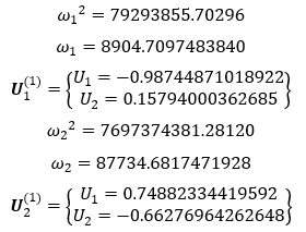
The square root of the diagonal matrix ![]() is also a diagonal matrix
is also a diagonal matrix ![]() with square root of eigenvalues
with square root of eigenvalues ![]() , that is the natural frequencies of the blade on the main diagonal.
, that is the natural frequencies of the blade on the main diagonal.
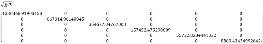
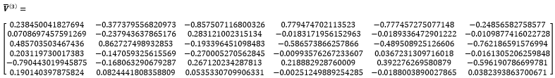
It is seen from ![]() that the fundamental natural frequency is ω1=8863.43434993196 rad/s with the corresponding eigenvector as the sixth column of V ̅(3) . The fundamental mode of the blade corresponding to the fundamental natural frequency is ω1 is a plot of the sixth column of V ̅(3) as shown in figure4.4.
that the fundamental natural frequency is ω1=8863.43434993196 rad/s with the corresponding eigenvector as the sixth column of V ̅(3) . The fundamental mode of the blade corresponding to the fundamental natural frequency is ω1 is a plot of the sixth column of V ̅(3) as shown in figure4.4.
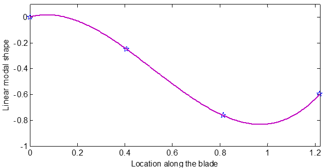
Fig.4(a). The fundamental Mode shape of the three-element rotating beam. (Linear mode shape)
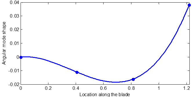
Fig. 4(b). The fundamental Mode shape of the three-element rotating beam. (Angular mode shape)
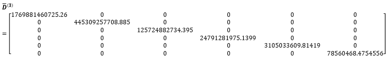
Following similar procedure, the diagonal matrix of eigenvalues ![]() of the matrix
of the matrix ![]() is computed as
is computed as
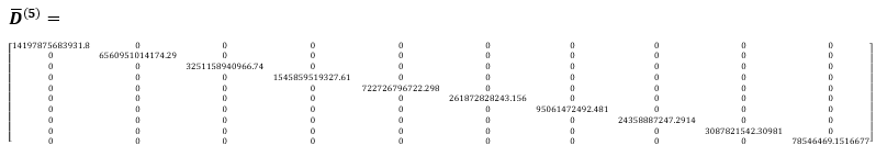
The corresponding diagonal matrix containing the natural frequencies becomes
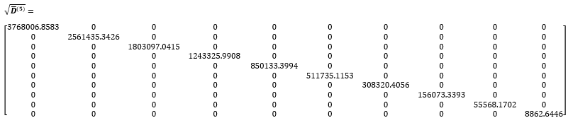
It is seen that the fundamental natural frequency of the five-element model is ω1=8862.64459129822 rad/s. this is given in four decimal places as seen in ![]() to be ω1=8862.6446rad/s. The corresponding fundamental eigenvector is {-0.070236&-0.0019302&-0.232762&-0.003277&-0.46043&-0.004058&-0.721594&-0.004385&-0.455875&0.017971}T. The fundamental mode shape is shown in fig. 5(a) and fig. 5(b).
to be ω1=8862.6446rad/s. The corresponding fundamental eigenvector is {-0.070236&-0.0019302&-0.232762&-0.003277&-0.46043&-0.004058&-0.721594&-0.004385&-0.455875&0.017971}T. The fundamental mode shape is shown in fig. 5(a) and fig. 5(b).
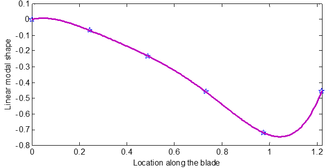
Fig. 5(a). Mode shape of the five-element rotating beam model. (Linear mode shape)
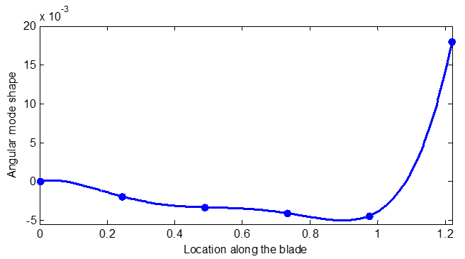
Fig. 5(b). Mode shape of the five-element rotating beam model. (Angular mode shape)
A good degree of agreement is seen between the mode shapes of the three and five-element models. This is an indication of validity of analysis. The fundamental natural frequency of the one, three and five-element models are ω1=8904.7097, ω1=8863.4343 and ω1=8862.6446. Fast rise in accuracy with increase in number of elements is seen. Relative to the five-element model the accuracy of the one and three-element models are respectively 0.47463% and 0.00891%. It is seen from these percentages that the one-element model is relatively accurate meaning that the three and five-element models can be considered accurate. Since the studied blade rotates at Ω=300 rpm which translates to circular frequency of ϖ= 31.4159 rad/s the problem of resonance during start-up is precluded since the fundamental natural frequency of the system is higher than the excitation frequency. The question of degree of contribution of rotation to transient response of the blade needs to be addressed. If there was no rotation, The fundamental natural frequency of the one, three and five-element models respectively become ω1=8904.6427, ω1=8863.4056 and ω1=8862.6273. It is seen that the one, three and five-element models respectively compute slight increase in fundamental natural frequency due to rotation relative to that of the non-rotating blade as 0.0007524%, 0.000323% and 0.000195%. These percentages translate to mean that effect of rotation could be marginal meaning that rotational motion can be ignored under this condition. Suppose that the rotational speed were to be increased to Ω=300 rpm which translates to circular frequency of ϖ=314.159265 rad/s. The corresponding fundamental natural frequency of the one, three and five-element models are ω1=8911.34492, ω1=8866.27918, and ω1=8864.35757. A 900% increase in rotational speed respectively incurred 0.075267%, 0.032421% and 0.019523% increase in fundamental frequency relative to the non-rotating the one, three and five-element models. This can be seen to mean that ten times increase in speed leads to about hundred times increase in rotational contribution. It can be said in conclusion that rotational effects in finite element modelling of helicopter blade can be ignored at law rotational speeds but should be taken into account when the rotational speed is high.
- Validity of Calculations
One element model has been used to analyze rotating cantilever beam in the work [19]. The beam in the work [19] was subjected to a rotational velocity given in the relation ![]() such that
such that
![]() (41)
(41)
Inserting the numerical values of this work;le= 1.2192 m, E=70.5 GPa , I=4.162314256×10⁻³ and m=20.903184 kgm-1 in the modal matrix ![]() for the one element model (e=1) gives
for the one element model (e=1) gives
![]() (42)
(42)
The natural frequencies become
ω1=9326.1834200071 (43a)
ω2=87972.9503427093 (43b)
The calculated natural frequencies in the work [19] are given by
![]() (44a)
(44a)
![]() (44b)
(44b)
A good agreement is seen between the two computations pointing to validity of method and computational procedure of this work. The difference between the two stem from small number of decimal places used in the coefficient of in “(44)”. Further validation of this work is derived from ANSYS. The analysis of the beam is carried out in three stages in ANSYS. The stages are Pre-processing, Solution and Post-processing. The three steps are detailed as follows; the first step of pre-processing required creation of the cross-section as a rectangular area by dimension which is to be meshed and extruded. The material properties are then imputed through the link of material models. The 2-D element and a 3-D elements needed are define. The 2-D element is needed for the beam cross-sectional area while the 3-D element is needed to extrude the cross-section along with the geometry of the beam. Five elements are prescribed in the extrusion. The 2-D element used in this work is the Quad 4 node ( PLANE182) while the 3-D element is the Brick 8 node ( SOLID185). Two kinds of loads are then applied. The first load is furnished by the boundary condition of constrained junction between the beam and the body. The other load is supplied as the rotational velocity of the beam. The solution stage required solving the problem as modal analysis type of problem. The post-processor is then used to view the results and various animations of the mode shapes of the rotating beam as shown in fig.6(a), fig. 6(b), fig 6(c) and fig 6(d). It should be seen from figure that the natural frequency arising from ANSYS tally with the corresponding natural frequencies in the matrix ![]() . It should be noted that frequencies in fig. 4 to fig. 6(d) are given in Hz while those in the matrix
. It should be noted that frequencies in fig. 4 to fig. 6(d) are given in Hz while those in the matrix ![]() are given in rad/s. Thus frequency values in the figures should be multiplied to correspond with those in
are given in rad/s. Thus frequency values in the figures should be multiplied to correspond with those in ![]() .
.
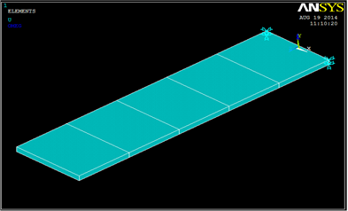
Fig 6(a) Solution of the studied rotational beam from ANSYS
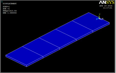
Fig 6(b) The first (fundamental) natural frequency [Hz] and mode shaped of the studied rotational beam
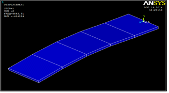
Fig. 6(c) The second natural frequency [Hz] and mode shaped of the studied rotational beam
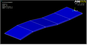
Fig. 6(d) (d)The fifth natural frequency [Hz] and mode shaped of the studied rotational beam.
CONCLUSION
Rotational effect on beam-finite element model of rotating cantilever is studied theoretically and validated with ANSYS simulation. The incremental stiffness matrix occasioned by rotation is derived using the principle of virtual work and given a generalized novel form that takes care of rotational stiffness contribution of any element in a multi-element model. The total stiffness matrix (sum of stiffness of non-rotating element and the rotational incremental stiffness matrix) is applied in the modal analysis of cantilever beam. Sensitivity analysis of the arising modal parameters to extent of discretization is carried out. The specific sensitivity results are given in what follows; One, three and five-element models where considered and fast rise in accuracy with increase in number of elements is seen. For example the fundamental natural frequency of the one, three and five-element models are respectively rad/s, rad/s and rad/s. This is interpreted to mean that relative to the five-element model the accuracy of the one and three-element models are respectively 0.47463% and 0.00891%. These percentages rather mean that the one-element model is relatively accurate meaning that the three and five-element models can be considered accurate. The one, three and five-element models respectively computed slight increase in fundamental natural frequency due to rotation relative to that of the non-rotating blade as 0.0007524%, 0.000323% and 0.000195%. The rotational speed is increased to rpm which translates to circular frequency of 314.159265 rad/s and it is seen that corresponding fundamental natural frequency of the one, three and five-element models are , , and . Thus a 900% increase in rotational speed respectively incurred 0.075267%, 0.032421% and 0.019523% increase in fundamental frequency relative to the non-rotating the one, three and five-element models. This can be seen to mean that ten times increase in speed leads to about hundred times increase in rotational contribution. In conclusion, rotational effects are marginal at low rotational speeds meaning that they can be ignored under this condition. Rotational effect should be taken into account when the rotational speed is high because rotational effect rises faster than rise of the causative rotational speeds.
REFERENCES
- E. Singh, and K. Gupta, “Free damped flexural vibration analysis of composite cylindrical tubes using beam and shell theories.” J Sound Vibration. 1994, 172(2)171–90.
- Kim, A. Argento, and R. A.Scott, “Free vibration of a rotating tapered composite Timoshenko shaft”. J Sound Vibration, 1999, vol.226(1), pp.25–47.
- Na, H. Yoon, and L. Librescu, “Effect of taper ratio on vibration and stability of a composite thin-walled spinning shaft”. Thin-Walled Structure, 2006, vol. 44, pp.62–71.
- Sino, T. N. Baranger, E. Chatelet, and G. Jacquet, “Dynamic analysis of a rotating composite shaft”. Compos Sci Technology, 2008, vol.68, pp. 37–45.
- Southwell, and F. Gough, “The free transverse vibration of airscrew blades,” British A.R.C. Reports and Memoranda, No. 766, 1921.
- Yntema, “Simplified procedures and charts for the rapid estimation of bending frequencies of rotating beams,” NACA 3459, 1955.
- Schilhansl, “Bending frequency of a rotating cantilever beam”, Journal of Applied Mechanics, 1958, vol.25, pp. 28–30.
- Carnegie, “Vibrations of rotating cantilever blading: theoretical approaches to the frequency problem based on energy methods”, Journal of Mechanical Engineering Science 1,1959, pp. 235–240.
- K. Chandiramani, L. Librescu, and C. D. Shete, “On the free-vibration of rotating composite beams using a higher-order shear formulation”. Aeros Sci Technology, 2002, 6, 545–61.
- Huang, W. Lin, and K. Hsiao, “Free vibration analysis of rotating Euler beams at high angular velocity”. Comput Structure, 2010, 88, pp. 991–1001.
- Vikas, A. Dhar, “Simple finite element for dynamic analysis of rotating composite beams: Master of Science thesis”, Virginia Polytechnic Institute and State University.
- P. Friedmann, “Helicopter Vibration Reduction Using Structural Optimization With Aeroelastic/Multidisciplinary Constrains – A Survey”, Journal of Aircraft, Vol. 28, No. 1, January 1991, pp. 8-21.
- Ganguli, and I.Chopra, “Aeroelastic Optimization of an Advance Geometry Helicopter Rotor”, Journal of the American Helicopter Society, Vol. 41 (1), January 1996, pp. 18-28.
- Phuriwat, “Semi-active control of helicopter vibration using controllable stiffness and damping devices.” PhD thesis: The Pennsylvania state university, 2002.
- C. Ihueze, P. C. Onyechi, H. Aginam, and C. G. Ozoegwu, “Finite Design against Buckling of Structures under Continuous Harmonic Excitation,” International Journal of Applied Engineering Research, 2011,6(12), pp.1445-1460.
- C. Ihueze, P. C. Onyechi, H. Aginam and C. G. Ozoegwu, “Finite Design against Buckling of Structures under Continuous Harmonic Excitation,” International Journal of Applied Engineering Research, ISSN 0973-4562 V, 6(12), (2011), pp. 1445-1460.
- S. Rao, “Mechanical Vibrations (4th ed.)”, Dorling Kindersley, India, 2004.
- John, “Introduction to Engineering Materials (3rd ed.)”, Palgrave, Hampshire, 1992, p.3.
- T. Thompson, and M. D. Dahleh, “Theory of vibration with applications (5th ed.)”. Prentice Hall, upper saddle river, New-Jersey.