
Time Series Analysis for Erosion Monitoring
- Ikediuwa, Udoka Chinedu
- Nnabude, Chinelo Ijeoma
- Osuji, George Amaeze
- Ndibe, Ifeoma Maryanne
- 303-309
- Jun 14, 2024
- Mathematics +1 more
Time Series Analysis for Erosion Monitoring
Ikediuwa, Udoka Chinedu, Nnabude, Chinelo Ijeoma, Osuji, George Amaeze, Ndibe, Ifeoma Maryanne
Department of Statistics, Nnamdi Azikiwe University Awka, Anambra State, Nigeria.
DOI : https://doi.org/10.51584/IJRIAS.2024.905027
Received: 06 May 2024; Accepted: 13 May 2024; Published: 14 June 2024
ABSTRACT
Erosion monitoring can range from small-scale, localized initiatives on a farm to large-scale regional or national monitoring programme. It is essential for encouraging the wise management of natural resources and sustainable land use. It is necessary to safeguard water quality, preserve soil fertility, preserve the stability of infrastructure and landscapes, and protect the environment. The Monitoring and Prediction of water quality are important in erosion management. Time series analysis was used in the monitoring of Erosion. The performance of time series statistical models were evaluated to predict and forecast on the factors that helps in monitoring erosion which include: Rainfall, Topography, Land use and Soil fertility menace from January 2013 to December, 2022.with the regression model: Mot = β0 + β1 R + β2 T + β3 LU + β4 SF + εt The Trend and Seasonal effects with the time correlation were also examined. The data were simulated and the results for the period of one year (January, 2022 to December, 2022) using trend and seasonal components showed sinusoidal wave. Also the results from the two components for the period of ten years (January, 2013 to December, 2022) showed oscillatory movement. From the results of the analysis carried out, and the predicted values obtained, erosion menace is highly predictable in the year 2024 and it is advised that precautionary measures should be taken in order to militate against this.
INTRODUCTION
The technique of methodically evaluating and tracking the eroding of land, soil, and natural landscapes over time is known as erosion monitoring. The process by which wind, water, ice, and other environmental elements erode away and reshape the Earth’s surface is called erosion. Additionally, human activities like building, agriculture, and deforestation might speed it up. There are several reasons why erosion monitoring is important, such as land management, disaster relief, and environmental conservation. To assess and analyze the pace, extent, and impact of erosion on a specific area and devise plans to prevent or manage its consequences, this procedure usually entails the use of a variety of methodologies and technologies. Sustainable land use, soil conservation, and erosion monitoring all depend heavily on erosion monitoring. Any activity caused by water in any form rain, flood, or sea that results in soil erosion is referred to as soil erosion. The loss of nutrients from the soil, which results in low agricultural yield, the destruction of farms, which causes building collapses, and the consequent homeless population are socioeconomic issues brought on by soil erosion. Yi Huang et. al (2019), present a technique and erosion corrosion monitoring sensor for real-time corrosion and erosion rate monitoring in electrolytic media environments. Fabien et. al (2020) in their article describes a monitoring system that locates and identifies erosion occurrences using distributed temperature sensing (DTS).
The goal of time series analysis is studying data gathered over time to identify trends, patterns, and variances in erosion processes. it is a potent and popular statistical technique for erosion monitoring. It offers insightful information about the temporal dynamics of erosion, which aids in decision-making and the application of efficient erosion control strategies by researchers and land managers. In order to comprehend the dynamic nature of erosion processes over time, time series analysis is essential in erosion monitoring. In addition to helping to create efficient erosion control and mitigation plans that safeguard the environment and promote sustainable land resource management, it offers a scientific basis for well-informed decision-making.
Time series analysis is crucial because it can identify patterns in variables observations, which improves forecasting ( Chatfield, 2004). when examining time series, it is best to begin with graphical representations to find series properties that are visible by looking at the plot of time series (Box and Jenkins, 1994).
According to Chatfield (2004). The division of observed times series into components that represent the trend (Tt) , the Season (St), cyclic ( Ct) and irregular (et) components is known as decomposition of time series. The trend briefly incorporates a cyclical component and the observed time series(Xt ∶ t = 1,2,⋯,n) can be broken down into seasonal (St), irregular (et) and trend – cycle components. Decomposition models are typical additive or multiplicative but can also take other form such as pseudo- mixed model (combination of the additive and multiplicative model).
Additive model:
Xt = Mt + St + et (1)
Multiplicative model :
Xt = Mt + St + et (2)
Mixed model :
Xt = Mt + St + et (3)
For the additive model and mixed models is assuming that the error component is a Gaussian N(0,σ2) white noise. While for multiplicative model it is assumed that et is the Gaussian N(1,σ2) white noise and cov (vt,vt+k) = 0, ∀ k ≠ 0 . The assumption in additive model is that the sum of the seasonal component over a complete period is zero.
∑j=1s Sj = 0 (4)
While for the multiplicative and mixed models is assuming that the sum of the seasonal component over a complete period is s.
![]() (5)
(5)
METHODS
We used the structural , the ARIMA and the time series regression models in this investigation. Especially, Harvey (1984, 1985) and Harvey and Durbin (1986), who examined a group of structural models constructed in the manner described below
Yt = μt + γt + et (6)
Where μt is trend, γt is seasonal, et is irregular components.
For trend we have
μt = α + βt + et (7)
The approach for the seasonal component ( with s seasons) is the trigonometric version defined in Harrison (1965) scheme. When s = 2m or 2m+1 according as even or odd.
![]() (8)
(8)
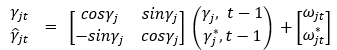 (9)
(9)
For j = 1, ⋯,m. with γ ̂mt = 0 for s even. In the basic structural model it is assumed that all the errors are normally distributed with constant variance
![]()
Comparing the structural models, which provide explicit interpretations through component breakdown, ARIMA models have the advantage of a stronger model building paradigm. Comparing the two models to regression models that disregard temporal structure or the rudimentary filtering of polynomial trends reveals significant improvements. The residuals from fitted values have been found to be generally unreliable as the basis for evaluating methods since a particular model may fit historical data well but be unreliable for extrapolation purposes. Therefore, the best way to assess the reliability of a forecasting method is to work at its performance over a period of time beyond that which the model was fitted (Kendall and Ord, 1990).
2.1 Time Series Regression Model
The mathematical time series regression model is represented as
![]() (10)
(10)
Where β1,β2,β3 and β4 are parameters to be estimated,then β0 is the intercept and εt is the error associated with the model assumed to be noise.
Mot=Erosion monitoring at time (t), R, T, LU and SF are the factors associated with the erosion.
R = Rainfall, T = topography, LU = Land use and SF = Soil fertility.
2.2 Regression with Auto-regressive Integrated Moving Average (ARIMA)
If the error term or the residual in equation (10) contains auto- correlation then εt is replaced by an error series φt that is assumed to follow ARIMA model. If all the variables in equation n(10) are stationary, then the ARIMA error will be considered also in applying differencing, then an ARIMA error is required ( Harris & Sollis, 2003). The time series multiple regression models with error series φt are written as
![]() (11)
(11)
For the time series regression model containing an ARIMA (p, d, q) errors, the φt is written as
![]() (12)
(12)
Where φt ~𝑖id (0, σε2 ), θ1,⋯,θp are the parameters of auto correlation (AR) errors that are to be estimated,γ1 ,⋯,γq are the parameters of the moving average (MA) error parts to be estimated.
RESULTS
Structural model, the ARIMA model and time series techniques were used to investigate the simulated erosion data. We assess the reliability of a forecasting method to look at the performance of the monitoring of erosion over a period of time.
The tabular results and graphical results are presented below.
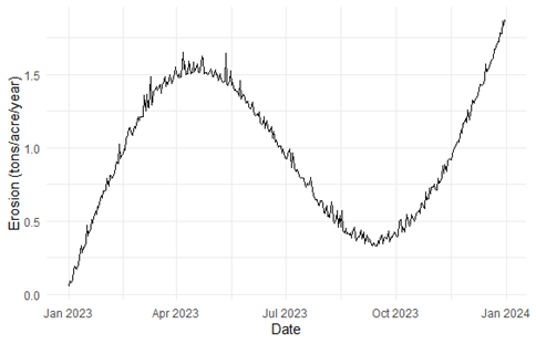
Fig 3.1: the graph of the erosion time series for one year
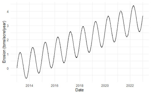
Fig 3.2: the graph of erosion time series for the period of ten (10) years
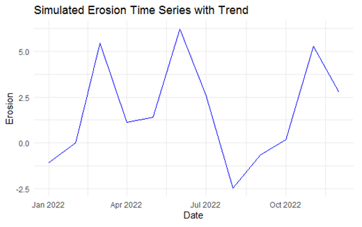
Fig. 3.3 The trend for the period of one year
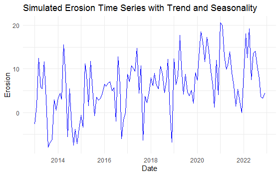
Fig 3.4 The graph of the trend and seasonality of the erosion simulated data
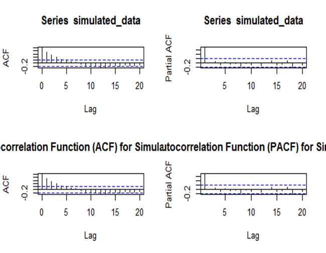
Fig 3.5: Auto Correlation and Partial Auto Correlation Functions of the simulated erosion data
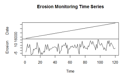
Fig. 3.6. The simulated auto correlation process
The residual standard error: 0.9794 95 degrees of freedom. R2 = 0.9691 .
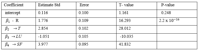
Table 3.1: The summary of the estimated values of the Time series Regression model.
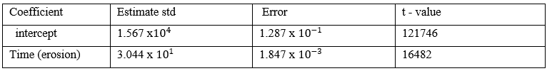
Residual standard error : 0.7008 0n 118 df, R2 = 1
Table 3.2: the residual and response of the trend analysis results
| month | forcast | 95% lower bound | 95% upper bound |
| JAN | 6280.14 | -231.15 | 12791.43 |
| FEB | 6263.72 | -249.82 | 12779.29 |
| MAR | 6252.38 | -268.11 | 12772.87 |
| APR | 6242.51 | -286.69 | 12771.71 |
| MAY | 6234.62 | -305.73 | 12775.09 |
| JUN | 6228.30 | -325.73 | 12782.32 |
| JUL | 6223.24 | -346.29 | 12792.78 |
| AUG | 6219.20 | -367.49 | 12805.89 |
| SEP | 6215.97 | -389.25 | 12821.18 |
| OCT | 6213.38 | -411.46 | 12838.22 |
| NOV | 6211.31 | -434.06 | 12856.68 |
| DEC | 6209.65 | -456.95 | 12876.26 |
Table 3.3. Forecast using Regression with ARIMA (0,0,1) model
Fig.3.1 The graph of the erosion time series for one year showed sinusoidal wave, with an upward swing in the first and second quarter meaning that there is more effect of erosion on the first and second quarter of the year while it has a low swing at the third quarter which showed there is less effect of erosion on the third quarter of the year.
Fig.3.2. The graph of the erosion time series for the period of ten years showed the characteristic patterns of seasonal variation on a rising trend.
Fig. 3.3 show an upward trend in the first quarter, fall in the second quarter, rise in the third quarter and falls too low in between the third and the last then rises again.
Fig.3.5 and 3.6 are the correlo gram of the simulated erosion data which showed that the series is stationary.
Table .3.1 and 3.2 showed the estimated erosion from the time series regression model which is given by Mot=0.116+1.776R+2.854T-1.051 LU+3.977 SF+et
Table 3.3 show monthly forecast for one year of the simulated data using ARIMA (0,0,1)
CONCLUSION
This paper focuses on erosion monitoring using time series analysis. The simulated erosion data was generated from the period of 2013 – 2022: Rainfall, Topography, Land use and Soil Fertility were chosen as the determinant factors of erosion. Regression model and structural models were obtained which showed that the models are adequate for erosion monitoring. The auto correlation function and partial auto correlation function were carried out which was used in checking the stationarity of the model. Regression with ARIMA was modeled which was used for the forecasting of the erosion. The results of the forecast showed that erosion is highly predictable especially in January 2024, in conclusion it is advised that precautionary measures should be taken in order to mitigate against this or consequences.
REFERENCES
- Box, G.E.P. Jenkins,G.M. and Reinsel, G.C. (1994). Time Series Analysis: Forecasting and Control. 3rd Edition,Prentice Hall, Englewood Cliff, New Jersey.
- Chatfield,C. (2004). The Analysis of Time Series: An Introduction. 6th Edition, Chapman and Hall/CRC Press, Boca Raton London
- Fabin, R., Christian, S., Rodolfo, G., Simo, M. and Etienne, R. (2020) “Erosion Risk Mitigation with DTS Based Monitoring System” https:\\doi.org\10.2118\202654-MS.
- Harvey, A.C.(1984).A unified view of statistical forecasting procedures. J Forecasting, 3, 245-275.
- Harvey, A.C and Durbin, J.(1986). The Effects of Seat Belt Legislation on British Road Causalities: A Case Study in Structural Time Series Model (with Discussion). J Roy. Statist. Soc. A. 149. 187-227
- Kendall, M. and Ord, J.K. (1990) “Time Series” Third Edition. Published by Halsted Press an imprint of John Wiley and Sons Inc, 605 Third Avenue New York, NY 10158.
- Monteiro,M. and Costa, M.(2018). A Time Series Model Comparison for Monitoring and Forecasting Water Quality Variables. Hydrology , 5(3), 37. https://doi.org/10.3390/hydrology5030037.
- Uchegbu, S.N, Ozulumba, .C., Ejikeme, .K., Andrew, .O., Andrew, .O., Christopher, .A., Obi, .N.I., Emeasoba, U.I., Agwuna, K.K. and Iroegbu,.A. (2004) “Soil Erosion in Awka, Anambra State(Nigeria)Assessing the Social and Environmental Effects” https:\\eprints.gouni.edu.ng
- Yi, .H., Liang, .L., Yunze, .X. and Xiaona, .W. (2019) “Erosion Corrosion Monitoring Sensor and Monitoring Method” https:\\typeset.10\papers