Sedimentological Analysis and Depositional Environmental Interpretation of Benin Formation: A Case Study of Umuaka and its Environs in Njaba Local Government Area, Imo State, Nigeria.
- Anumaka, C.C.
- Anozie, H.C.
- Ahaneku, C.V.
- Okpara, A.O.
- Odinye, A.C.
- Onuchukwu, E.E.
- Oshim, F.O
- 492-509
- Jul 19, 2024
- Environment
Sedimentological Analysis and Depositional Environmental Interpretation of Benin Formation: A Case Study of Umuaka and its Environs in Njaba Local Government Area, Imo State, Nigeria.
Anumaka, C.C., Anozie, H.C., Ahaneku, C.V., Okpara, A.O., Odinye, A.C., Onuchukwu, E.E. and Oshim, F.O
Nnamdi Azikiwe University, Awka, Nigeria
DOI : https://doi.org/10.51584/IJRIAS.2024.906044
Received: 27 May 2024; Revised: 12 June 2024; Accepted: 17 June 2024; Published: 19 July 2024
ABSTRACT
The study of sedimentology is an important interdisciplinary field that helps us understand Earth’s history, environmental processes, and natural resources. This research focused on analyzing the characteristics of coastal sediments in the Umuaka area of Njaba Local Government Area in Imo State, Nigeria. The goal was to determine the source of the sediments, the environment in which they were deposited, and the processes that shaped the coastal landscape. The study area lies between latitudes N 50 38′ 11.5” and N 50 42′ 3.6” and longitudes E 70 4′ 4.9” and E 60 59′ 0.0”, with an altitude of 31 m to 160 m above sea level. The topography is characterized by hilly highlands and lowlands with sparse vegetation and gallery forests along the river channels. Access is via the Orlu – Owerri highway. The study area is in the Niger Delta Basin and is underlain by the Benin Formation. Methodology included desk research, reconnaissance, detailed geological field mapping and laboratory analysis. Field mapping revealed that the rock consists of friable, highly stratified, fine to very coarse sandstone with intercalations of clay/mudstone. Grain size analysis revealed that the sandstones were fine to very coarse grained ɸ(2.58 to -0.70)), moderately to poorly sorted ɸ(1.43 to 0.53), very positive to very negative skewness (0, 45 to – 0.63)). and leptokurtic to platykurtic (1.42 to 0.67). The predominant physical sedimentary structures identified were planar cross-bedding and graded beds, while the biogenic structures were dominated by vertical Skolithos caves. The bivariate and multivariate analyses, as well as the structural, physical and biogenic structures, indicate that the sediments were predominantly deposited in a shallow marine beach environment. The predominant process of sediment accumulation was through turbidity current deposition, with little influence from fluvial processes. Further studies are recommended to monitor and evaluate coastal sediment dynamics in response to ongoing natural and anthropogenic changes.
Keywords: Benin Formation, sedimentological analysis, textural characteristics, paleocurrent analysis, sedimentary structures, paleoenvironmental analysis, Umuaka, Imo State.
INTRODUCTION
The study of sedimentological rocks and their associated processes has been a cornerstone in understanding Earth’s geological history and understanding past environmental conditions. Analysis of grain size distribution has been widely used by sedimentologists to classify sedimentary environments and elucidate transport dynamics (Ayodele, and Madukwe, 2019). The study area selected for this research is a region of significant geological interest, characterized by a variety of geological features, landforms, and rock types. The unique geological features observed in this area provide a valuable opportunity to study the geological processes and evolutionary history that have shaped it over geological time periods. The environmental interpretation of grain size distribution found in sedimentary deposits has been still a fundamental goal of sedimentlogy (Venkatesan and Singarasubramanian, 2016). The Benin Formation, a major geological unit in the Umuaka area of Njaba Local Government Area of Imo State, provides a fascinating opportunity to explore the sedimentological characteristics, depositional environment and underlying processes that contributed to the formation of this unique geological layer. The Umuaka region is a witness to the dynamic interplay of natural forces and environmental conditions that has resulted in the deposition and subsequent transformation of sediments over the centuries.
LOCATION, GEOMORPHOLOGY AND GEOLOGY OF STUDY AREA
The study area is in Umuaka, which is part of the Njaba Local Government Area in Imo State, Southeastern Nigeria. It lies between latitudes N5°38’11.5” and N5°42’3.6” and longitudes E7°04’4.9” and E6°59’0.0” (figure 1). The town has a relatively high population density, estimated to be over 40,000 people according to the National Population Commission in 2006.
The area being studied has rolling hills and the highest point is about 340 meters above sea level (Ofoegbu et al., 2019). The land surface is dominated by a steep slope that serves as a drainage channel to the nearby rivers and streams (figure 2). These local rivers are tributaries to the Njaba River which eventually flows into Aguta Lake. The erosion and weathering of the high and lowlands have formed a wave-like land structure. The hilly topography has sparsely positioned gully sites that resulted from the erosion of sand Formation (Benin formation) characterized by friable sand, fissile shale, and sandy shale (Nwajide, 2004).
The topography of the Umuaka area and its environs is characterized by undulating hills with spares vegetation and valleys with gallery forest along drainage lines, with the major landform being the Orlu-Umuna-Umuduru hills, which rise to about 400 meters above sea level mainly made of sandstone and subordinate clay (Ihekaire, 2016). The drainage pattern of the study area is dendritic, and it has a good drainage system that controls run-off (figure 3).
The area is in Niger Delta Basin. This sedimentary basin in the study area was deposited during Eocene to recent. The three key formations/stratigraphic units within the Niger Delta basin are the bottom Akata, middle Agbada and topmost Benin Formations. The study area is underlained by Benin Formation of Miocene-recent (figure 4). The Benin Formation extends from the west across the whole Niger Delta and southward beyond the present coastline. It consists of very friable sand and sandstones, and lenses of clay and shale (Short and Stauble, 1967). The Benin Formation is thus partly marine, partly deltaic, and partly estuarine, and is underlain by paralic Agbada Formation (Oligocene) and pro-delta Akata Formation (Eocene-Recent) (Reyment, 1965). According to Ojo and Tsalides (2014), the Benin Formation is the second-most important petroleum reservoir rock in the Niger Delta Basin after the Agbada Formation.
Benin Formation is the first, newest, coastal plain, Miocene to Recent Benin Formation (Short and Stauble 1967; Evamy et al. 1978; Ejedawe 1986; Doust and Omatsola 1990) largely comprises of deposits of alluvia and non-marine sand stones, in a continental, yet fluvial setting, engulfing the western flank of the Niger Delta complex to the total basin and the southern region of the shoreline. Bands of gravel lignite, wood fragments, minute intercalations of shales and coarse- grained sandstones are prime deposits observed. It is also primarily linked with infinitesimal accumulation of hydrocarbon (Akanji et al., 2018). The thickness of this Formation varies widely, surpassing 1820 m in some instances. It is characterized by high porosity and permeability, making it an ideal host for hydrocarbon accumulation. Several studies have been conducted to understand the geology and sedimentology of the Benin Formation, and to explore its hydrocarbon potential (Iwuagwu et al., 2017; Olatunji et al., 2018).
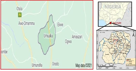
Fig 1: Map showing the study area
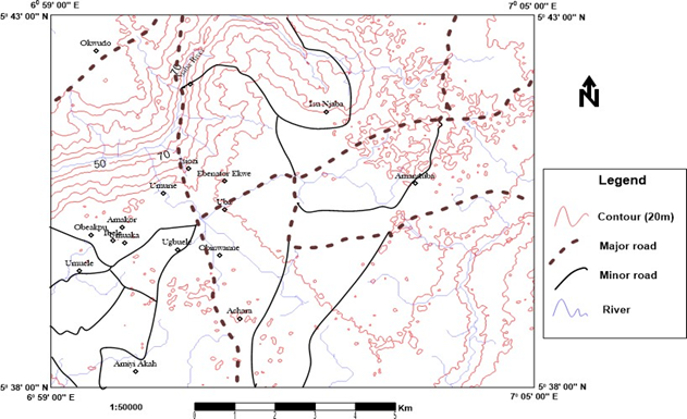
Fig 2: Topographic map of the study area.
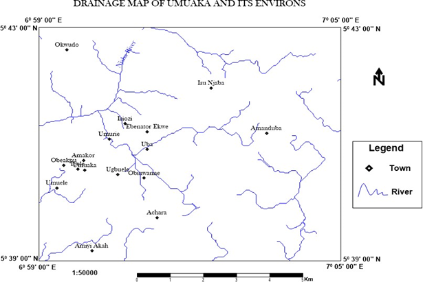
Fig 3: Drainage map of the study area showing the flow pattern.
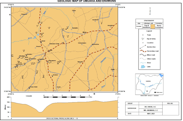
Fig 4: Geologic map of the study area
MATERIALS AND METHODS
Bearings were determined using the Geographic Positioning System (GPS) and a compass. Several geological and software materials were used in this project. The investigation began with a proper review of pre-existing literature relevant to the study area, planning, desk study, reconnaissance survey, detailed geological field mapping and laboratory analysis. Detailed geological mapping was carried out by logging the outcrop, identifying the location of the strata at a particular site or station, the outcrop, trend of the outcrop/station, considering the rock type/lithology of the rock samples and the structural characteristics of the rock samples. Outcrop sections of the study area were described in terms of lithofacies parameters such as lithology, sedimentary structures (physical and biogenic), texture and bed thickness. The exposed outcrops were clearly described. The locations of the outcrops were marked on the map. The paleocurrent direction of the study area was derived using structures. Bearing the dip directions of the crossbeds was used to infer the direction of paleocurrents of the sand deposits. Paleocurrent data were plotted in a rose diagram using the Georose software application. Samples were also collected for analysis and interpretation. During the field mapping, 43 locations were visited, as shown on the geological map above. 23 sand samples were collected for texture analysis. This method was used to calculate the grain size of the sediment and determine the depositional environment. The classification of the samples is based on the grain size distribution and the proportion of particles of different sizes in the sample. The collected samples were sieved (using a ½ phi interval sieve mesh (ASTM)) on a digital sieve machine for a period of at least 15 minutes, and then the results were described and interpreted using Folk and Ward (1957) Inclusive Graphic Measures and statistical parameters of grain size such as mean, standard deviation, skewness and kurtosis were calculated using the critical percentile from the cumulative frequency plots. The data obtained from sieve analysis of the collected samples were used to calculate the following using Folk and Ward’s (1957) formula and terms and scale (Table 1): (mode, median, mean, standard deviation (sorting), kurtosis and skewness).
Mean = ∅16+∅50+∅84……………………………………………………………………………………………………………………. (1)
3
Standard deviation (sorting) = ∅𝟖𝟒−∅𝟏𝟔 + ∅𝟗𝟓−∅𝟓……………………………………………………………………………………………………………………. (2)
𝟒 𝟔.𝟔
Median = ∅50……………………………………………………………………………………………………………………. (3)
Skewness = ∅16+∅84−2∅50 + ∅5+∅95−2∅50……………………………………………………………………………………………………………………. (4)
2(∅84−∅16) 2(∅95−∅5)
Kurtosis = ∅95−∅5……………………………………………………………………………………………………………………. (5)
2.44(∅75−∅25
Where ∅5, ∅16, ∅25, ∅50, ∅75, ∅84 and ∅95 represents 5th, 16th, 25th, 50th, 75th, 84th and 95th percentile, respectively, on the cumulative curve. (Folk and Ward, 1957)
Paleoenviromental Analysis Parameters
The multivariate discrimination functions (Y1, Y2, Y3 and Y4) proposed by Sahu (1964) were applied to the grain size analysis data to characterize the depositional environment and deposition of sediments from the study area. Paleoenvironmental analysis was performed using bivariate and multivariate functions.
Y1 (Aeolian beach) = -3.5688(Mean) +3.7016 (Standard Deviation)2 – 2.0766(Skewness)
+3.1135(Kurtosis)………………………………………………………………………….. (6)
Y2 (beach: shallow marine) = 15.6534(Mean) – 8.7604 (Standard Deviation)2 – 4.8932 (Skewness) + 18.5043 (Kurtosis)………………………………………………. (7)
Y3 (shallow marine: shallow agitated) = 0.2852(Mean) – 8.7604(standard deviation) 2 – 4.893(Skewness) + 0.0482 (Kurtosis)…………………………………………………. (8)
Y4(Fluvial: Turbidity Current) = 0.7215(Mean) − 0.4030(Standard Deviation)2 + 6.7322(Skewness) + 5.2927(Kurtosis)………. (9)
If Y1 greater than (>) -2.7411, then the environment of deposition falls within beach and less than (<) the number described it is Aeolian.
If Y2 < 65.6534, then beach conditions are confirmed. If Y2 > 65.6534, then shallow agitated conditions are expected
If Y3 > -7.4190, shallow marine environment confirmed. If Y3 < -7.4190, fluvial environment indicated.
If Y4 is < 9.8433, it indicates turbidity current deposition and if Y4 is > 9.8433, it indicates deltaic deposition.
RESULTS AND DISCUSSION
Textural Characteristics
From the calculated statistical parameters (Tables 2 and 3) it can be deduced that the sand samples from the study area are predominantly fine-grained to very coarse-grained based on their mean values. The standard deviation representing the sorting of the grains shows poor to moderate sorting. It can be deduced or concluded that most of the sand units in the area were deposited on beaches with little influence from fluvial environments, just not too far above the continental shelf, as poorly to moderately sorted sands represent sands found in rivers, lagoons and distal marine areas Shelf and subinland dune depositional environments. The kurtosis values showing that the peak of the distribution curve is platykurtic, leptokurtic and leptokurtic. The Skewness, which is the most important parameter in environmental discrimination, has values that are mostly negative showing that the samples are negatively skewed. which is typical of marine sands across the continental shelf. Majority of the coarse and fine sands are poorly sorted to moderately sorted while the medium sands are dominantly moderately sorted. Most of the sands lie within near symmetrical, positively skewed, negatively skewed, and very positively skewed. The sand collected lies within mesokurtic, platykurtic and leptokurtic. This suggests the dominance of coarse-grained size population which is responsible for the positive skewness and the presence of a subordinate population of medium grained sands. The negative skewness of the sediments is attributed to higher energy conditions. The kurtosis for Benin Formation revealed leptokurtic to platykurtic, which suggests that Benin Formation were sourced from more than one sources. This show that Benin Formation was deposited in a shallow marine beach setting with prevalent of turbidity and fluvial processes. The fissility and the fine nature (Grainsize) of the intercalation of fine grain (clay) in Benin formation as indicated by the field data suggest also that the sediments were deposited below the wave base, accumulated in relatively low energy environment i.e., in a distal to proximal lagoon but mostly fluvial environment. Thus, the variation in the wave energy could also be rresponsible for the variation in the particle sizes (the medium and the coarse variations) in the Benin Formations. Presences of interaction of mudstone units within Benin Formation sequence indicates a quiet environment with very low energy
Table 2: Summary of the calculated statistical parameter for all the 23 samples
| No | Mean (∅) | Median (∅) | Kurt | StD (∅) | Skew | Remark |
| S 1 | 0.60 | 0.47 | 0.90 | 1.37 | 0.10 | Coarse grained sand, poorly sorted, mesokurtic, and nearly symmetrical |
| S 2 | 0.44 | 0.48 | 1.08 | 1.11 | -0.04 | Coarse grained sand, poorly sorted, mesokurtic, and nearly symmetrical |
| S 3 | 0.75 | 0.62 | 0.84 | 1.28 | 0.09 | Coarse grained sand, poorly sorted, platykurtic, and positively skewed |
| S 4 | 1.23 | 1.28 | 1.15 | 0.68 | -0.04 | Medium grained sand, moderately sorted, leptokurtic, and nearly symmetrical |
| WS B | 0.62 | 0.63 | 0.95 | 1.07 | -0.01 | Coarse grained sand, poorly sorted, mesokurtic, and nearly symmetrical |
| WS A | 0.12 | -0.06 | 1.41 | 1.15 | 0.45 | Coarse grained sand, poorly sorted, leptokurtic, and very positively skewed |
| S 7 | -0.46 | -0.47 | 0.92 | 0.91 | -0.09 | very coarse-grained sand, moderately sorted, mesokurtic, and very negatively skewed |
| S 8 | 2.13 | 2.14 | 1.07 | 1.03 | -0.03 | Fine grained sand, moderately sorted, mesokurtic, and nearly symmetrical |
| S 9 | 1.53 | 1.41 | 1.02 | 1.15 | 0.18 | Medium grained sand, poorly sorted, mesokurtic, and positively skewed |
| S 10 | 2.58 | 3.14 | 0.70 | 1.30 | -0.63 | Fine grained sand, poorly sorted, platykurtic, and very negatively skewed |
| S 11 | 2.19 | 2.29 | 0.67 | 1.43 | -0.19 | Fine grained sand, poorly sorted, platykurtic, and negatively skewed |
| WS 1 | 0.48 | 0.42 | 1.05 | 0.90 | 0.15 | Coarse grained sand, moderately sorted, mesokurtic, and positively skewed |
| WS 2 | 0.07 | 0.03 | 0.97 | 0.72 | 0.19 | Coarse grained sand, moderately sorted, mesokurtic, and positively skewed |
| WS 3 | 0.45 | 0.41 | 1.05 | 0.92 | 0.13 | Coarse grained sand, moderately sorted, mesokurtic, and positively skewed |
| WS 4 | 0.42 | 0.41 | 0.99 | 0.77 | 0.07 | Coarse grained sand, moderately sorted, leptokurtic, and nearly symmetrical |
| WS 5 | -0.25 | -0.39 | 0.92 | 0.63 | 0.37 | very coarse-grained sand, moderately sorted, mesokurtic, and very positively skewed |
| WS 6 | -0.20 | -0.28 | 0.91 | 0.68 | 0.13 | very coarse-grained sand, moderately sorted, mesokurtic, and positively skewed |
| WS 7 | -0.29 | -0.43 | 0.86 | 1.00 | 0.26 | very coarse-grained sand, poorly sorted, platykurtic, and positively skewed |
| WS 8 | -0.52 | -0.67 | 0.86 | 0.89 | 0.33 | very coarse gained sand, moderately sorted, platykurtic and very positively skewed |
| WS 9 | -0.70 | -0.69 | 1.22 | 0.59 | 0.13 | very coarse-grained sand, moderately sorted, leptokurtic, and positively skewed |
| WS 10 | -0.06 | -0.04 | 1.21 | 0.72 | -0.01 | very coarse-grained sand, moderately sorted, leptokurtic, and nearly symmetrical |
| WS 11 | 0.75 | 0.87 | 1.12 | 0.53 | -0.20 | Coarse grained sand, moderately sorted, leptokurtic, and nearly symmetrical |
| WS 12 | 0.60 | 0.61 | 0.92 | 0.57 | 0.08 | Coarse grained sand, moderately sorted, mesokurtic, and nearly symmetrical |
StD – Standard deviation
S – Sample
WS – Well Sample Kurt- kurtosis Skew- skewness
Table 3: Summary of the interpretation of the textural characteristics
| Statistical parameters | Maximum value | Minimum value | Average | Range/remark |
| Mean (∅) | 2.58 | -0.70 | 0.54 | Fine to very coarse |
| Standard deviation (∅) | 1.43 | 0.53 | 0.93 | Poorly sorted to moderately sorted |
| Kurtosis | 1.42 | 0.67 | 0.99 | Platykurtic to leptokurtic |
| Skewness | 0.45 | -0.63 | 0.06 | Very positively skewed to very negatively skewed |
Paleocurrent Analysis
The rose diagram (fig 5) from the azimuths of the cross bed is bimodal and unipolar. The bi- directional paleo-flow suggest that sediments were transported from the southeastern or southwestern direction. From the analysis done, it was also seen that the cross beds were deposited in the Northwest direction. This shows that it was in a high energy environment. The paleocurrent analysis carried out, revealed that the sediments are flowing towards the northwest direction having its provenance probably from the southeastern or southwestern direction. Thus, the sediments were from the southern direction of the Benue Trough. This study has shown that the Benin formation is a product of fluvial transported and tidal current energy from Southern directions. The paleocurrent analysis suggests that the sediments were sourced from the southern Benue Trough. Benin formation has its origin linked to the succession of tectonic events that occurred in the Atlantic province during the late Cretaceous.
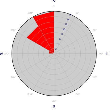
Fig 5: Rose diagram showing the paleocurrent direction of the cross beds
Sedimentary Structures
The sedimentary structure in rocks is used measurement of present-day rock geometries to uncover information about the history of deformation about the history of deformation in the rocks and ultimately to understand the stress field that resulted in the observed strain and geometries. The deformation of rocks could be syn-deposition or post-deposition. Syn- depositional structures are found at the time of deposition while post-depositional are secondary structures which are formed after the sediments have been deposited. Sedimentary structures observed in the study area are planer cross beds, graded beddings, mud cracks and biogenic structures such as vertical skolithos borrows. They are beds laid down at an angel to the horizontal, as in many sand dunes. Benin sandstone is cross bedded in confirmation of the nomenclature given to the formation with cross beds with first bed having its angle of inclination with underlying major bedding planes ranging from 40 to 130. Graded beds are formed from the systematic changes in grain size from the base of the bed to the top during sediment deposition. The changes are because of rise or drop in energy of deposition of transporting medium. Normal and inverse graded beds form as a current of water (ocean and stream) transporting a variety of sediments grains slow gradually, larger sediments grain settle first, followed by smaller grain as the current carrying capacity decreases. Thus, a typical normal graded bed has larger sediments grains at the bottom, with progressive smaller grains towards the top. Normal graded beds were seen Benin sand in the study area. Mud cracks are seen where denser lithologies are found overlying weaker formation or lithology as shown with an arrow (fig. 6D). The clay naturally shrinks when its losses moisture and expand when wet with moisture. This leads to large volume changes that generate enormous pressure upwardly, hence destroying structures found on it.
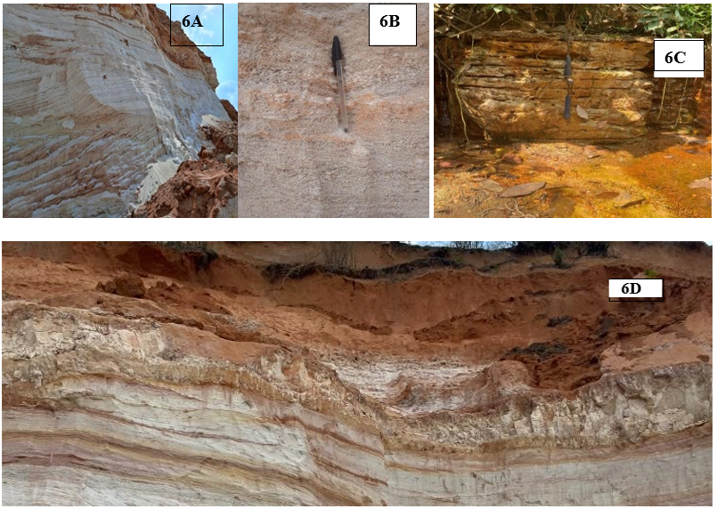
Fig 6: showing sedimentary structures in the study area (6A: Showing planar cross beds, 6B: showing graded bedding, 6C: mud cracks and 6D: showing biogenic structures).
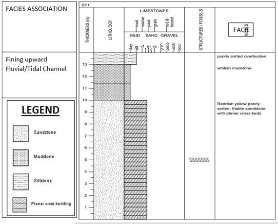
Fig 7: Lithologic section for mining site at Okwudor Near Njaba River
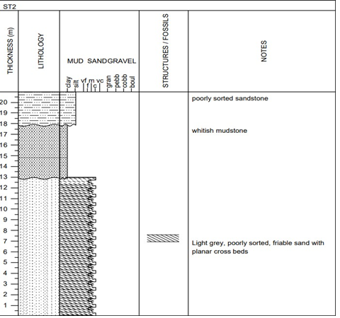
Fig 8: Lithologic section for mining site at Orlu Road Opposite Njaba River
Paleoenvironmental Analysis
From the multivariate and bivariate discriminate function, the environment of deposition is basically beach (96%) as almost all the calculated Y1 were deposited in Beach Environment.
While the Y2 calculated confirmed that they were deposited in Beach and shallow agitated condition expected. From the results of the calculated Y3 majority of the sands were deposited in fluvial environment while some indicates shallow marine environment (fluvial = 57%, shallow marine = 43%). From the calculated Y4, 96% of the sediments were transported and deposited by turbidity current. While 4% were transported and deposited by fluvial. This shows that the sediments were predominantly deposited in a shallow marine beach setting, where the dominant process of sediment accumulation was through turbidity current deposition (mechanism) with only a minor influence of fluvial processes. Within this coastal environment, the deposition of sediments was primarily driven by the action of turbidity currents. The resulting sedimentary deposits reflect the distinctive characteristics of a beach setting influenced by turbidity currents. The impact of fluvial processes on the sedimentation was minor, suggesting that the sediments primarily originated from local or nearby sources within the marine environment.
Table 4: Showing summery of the interpretation of the environment of deposition
| Number No | Y1 | Environment of deposition | Y2 | Environment of deposition | Y3 | Environment of deposition | Y4 | Depositional processes |
| sample 1 | 7.44 | Beach | 9.00 | Shallow agitated conditions are expected | -16.78 | Fluvial environment indicated | 5.11 | Turbidity current deposition |
| Sample 2 | 6.48 | Beach | 16.46 | Beach confirmed | -10.39 | Fluvial environment indicated | 5.26 | Turbidity current deposition |
| Sample 3 | 5.84 | Beach | 12.49 | Beach confirmed | -14.53 | Fluvial environment indicated | 4.91 | Turbidity current deposition |
| sample 4 | 0.99 | Beach | 36.78 | Beach confirmed | -3.46 | Shallow marine environment confirmed | 6.55 | Turbidity current deposition |
| Well Sample B | 4.95 | Beach | 17.25 | Beach confirmed | -9.70 | Fluvial environment indicated | 4.96 | Turbidity current deposition |
| Well sample A | 7.97 | Beach | 14.26 | Beach confirmed | -13.77 | Fluvial environment indicated | 10.08 | Fluvial (deltaic) deposition |
| sample 7 | 7.74 | Beach | 3.16 | Beach confirmed | -6.84 | Shallow marine environment confirmed | 3.59 | Turbidity current deposition |
| sample 8 | -0.26 | Aeolian | 43.95 | Beach confirmed | -8.51 | Fluvial environment indicated | 6.56 | Turbidity current deposition |
| sample 9 | 2.25 | Beach | 30.40 | Beach confirmed | -11.96 | Fluvial environment indicated | 7.20 | Turbidity current deposition |
| sample 10 | 0.50 | Beach | 41.67 | Beach confirmed | -10.90 | Fluvial environment indicated | 0.63 | Turbidity current deposition |
| sample 11 | 2.19 | Beach | 29.84 | Beach confirmed | -16.24 | Fluvial environment indicated | 2.99 | Turbidity current deposition |
| well sample 1 | 4.23 | Beach | 19.16 | Beach confirmed | -7.68 | Fluvial environment indicated | 6.66 | Turbidity current deposition |
| well sample 2 | 4.29 | Beach | 13.54 | Beach confirmed | -5.40 | Shallow marine environment confirmed | 6.28 | Turbidity current deposition |
| well sample 3 | 4.49 | Beach | 18.50 | Beach confirmed | -7.88 | Fluvial environment indicated | 6.47 | Turbidity current deposition |
| well sample 4 | 3.62 | Beach | 19.33 | Beach confirmed | -5.36 | Shallow marine environment confirmed | 5.76 | Turbidity current deposition |
| well sample 5 | 4.48 | Beach | 7.81 | Beach confirmed | -5.36 | Shallow marine environment confirmed | 7.03 | Turbidity current deposition |
| well sample 6 | 4.99 | Beach | 9.05 | Beach confirmed | -4.72 | Shallow marine environment confirmed | 5.41 | Turbidity current deposition |
| well sample 7 | 6.85 | Beach | 1.43 | Beach confirmed | -10.00 | Fluvial environment indicated | 5.68 | Turbidity current deposition |
| well sample 8 | 6.78 | Beach | -0.84 | Beach confirmed | -8.65 | Fluvial environment indicated | 6.03 | Turbidity current deposition |
| well sample 9 | 7.36 | Beach | 7.85 | Beach confirmed | -3.87 | Shallow marine environment confirmed | 6.67 | Turbidity current deposition |
| well sample 10 | 5.95 | Beach | 16.94 | Beach confirmed | -4.44 | Shallow marine environment confirmed | 6.06 | Turbidity current deposition |
| well sample 11 | 2.26 | Beach | 30.97 | Beach confirmed | -1.25 | Shallow marine environment confirmed | 5.02 | Turbidity current deposition |
| well sample 12 | 1.76 | Beach | 23.20 | Beach confirmed | -2.98 | Shallow marine environment confirmed | 5.69 | Turbidity current deposition |
CONCLUSION AND RECOMMENDATION CONCLUSION
The geology of the area as well as the structural parameters suggest that the depositional environment is predominantly in shallow marine beaches, where the dominant process of accumulation was by turbidity currents with little influence from fluvial processes. The appearance of caves suggests deposition in a high-energy intertidal and intertidal plain. The age of the sediments is Miocene-Pleistocene, with the beds dipping mostly in a northwesterly direction. The poorly to moderately sorted and friable nature of the study area suggested that the area is prone to erosion. This is because the sand is not cemented and is very susceptible to erosion.
Recommendation
- Stringent laws pertaining to mining operations need to be enforced by the government to combat erosion in the region, with corresponding regulations and penalties for violators being strongly advocated.
- Preventative measures must be taken to control sheet and rill erosion before they escalate into gullies.
- The entire study area should be surveyed using geotechnical methods to identify the areas prone to erosion and to construct appropriate drainage channels.
- Construction of suitable drainage channels to direct the water to a nearby surface water
Further studies are recommended to monitor and evaluate coastal sediment dynamics in response to ongoing natural and anthropogenic changes.
REFERNCES
- Akanji, A., Sanuade, A. O., Kaka, I. S. and Balogun, I. (2018) Integration of 3D Seismic and Well Log Data for the Exploration of Kini Field, Off-Shore Niger Delta. Petroleum and Coal 60(4), pp. 752-761.
- Ayodele, S., Madukwe, Y.(2019) Granulometric and Sedimentologic study of Beach Sediments, Lagos, Southwestern Nigeria. International Journal of Geosciences. Vol. 10 No.3
- Folk, K. C and Ward, W. C. (1957), the study in the significance of grain size parameters. journal of sedimentary petrology, vol.27, pp. 3-25.
- Ihekaire, C. U. (2016). Geographical information system (GIS) analysis of land use/land cover change in Umuaka, Imo State, Nigeria. Journal of Geography and Geology, 8(1), 84-91. doi: 10.5539/jgg.v8n1p84
- Iwuagwu, C. J., Ekweozor, C. M., & Akpan, U. G. (2017). Depositional environments and reservoir quality of the Benin Formation, Niger Delta Basin, Nigeria. Journal of African Earth Sciences, 134, 803-818.
- National Population Commission. (2006). “Population Census of the Federal Republic of Nigeria.” Abuja: National Population Commission.
- Nwajide, C. S., Reijers, T. J. A. (2004). A geological field excursion to parts of the Anambra Basin Nigeria, In: NAPE mini conference held at Federal University of Technology, Owerri 7-8 May 2004, pp1-28.
- Ojo, O. J., & Tsalides, P. (2014). Geology and hydrocarbon potentials of the Benin Formation in the Niger Delta Basin, Nigeria. Journal of Geology and Mining Research, 6(2), 21-34.
- Olatunji, A. S., Adekoya, J. A., & Ojo, T. A. (2018). Reservoir properties of the Benin Formation in the offshore area of the Niger Delta Basin, Nigeria. Journal of Petroleum Science and Engineering, 167, 419-432.
- Reyment, R. A. (1965). Aspects of the geology of Nigeria. Heinemann Educational Books.
- Sahu B. K. (1964). Depositional mechanism for sieve analysis of clastic sediments. Journal of sedimentology,vol. 34, pp 73-83.
- Short, K. C., & Stauble, A. J. (1967). Outline of geology of Niger Delta. American Association of Petroleum Geologists Bulletin, 51(5), 761-779.
- Venkatesan, S.V., Singarasubramanian, S.R and Suganraj.,K. (2016). Depositional mechanism of sediments through size analysis from the core of Arasalar river near Karaikkal, east coast of India. Indian Journal of Geo-Marine Sciencesvol. 34, pp 73- 83.
APPEDIX
Table 5. Summary of the calculated ɸ95, ɸ84, ɸ75, ɸ50, ɸ25, ɸ16, ɸ15, ɸ5
| No | phi95 | phi84 | Phi75 | phi50 | phi25 | phi16 | phi15 | phi5 |
| S 1 | 2.821928 | 2.067445 | 1.552984 | 0.470099 | -0.4539 | -0.74962 | -0.78248 | -1.58926 |
| S 2 | 2.316663 | 1.488692 | 1.155788 | 0.483707 | -0.27191 | -0.65382 | -0.69625 | -1.47672 |
| S 3 | 2.66985 | 2.172652 | 1.765854 | 0.622336 | -0.16358 | -0.54991 | -0.59664 | -1.28963 |
| S 4 | 2.531588 | 1.836162 | 1.688574 | 1.278606 | 0.826139 | 0.584468 | 0.548298 | 0.104107 |
| WS B | 2.405464 | 1.679808 | 1.427139 | 0.632842 | -0.09195 | -0.45811 | -0.50936 | -1.09814 |
| WS A | 3.434761 | 1.197252 | 0.68505 | -0.07587 | -0.58623 | -0.75516 | -0.77393 | -0.96163 |
| S 7 | 0.576046 | 0.567857 | 0.175557 | -0.46854 | -0.99445 | -1.46691 | -1.52035 | -2.05481 |
| S 8 | 3.72795 | 3.168337 | 2.726274 | 2.135051 | 1.437887 | 1.081021 | 1.035767 | 0.362883 |
| S 9 | 3.74 | 2.715072 | 2.312396 | 1.413012 | 0.77152 | 0.452293 | 0.415174 | -0.11004 |
| S 10 | 3.74 | 3.74 | 3.74 | 3.135315 | 1.485 | 0.873636 | 0.806818 | -0.09862 |
| S 11 | 3.74 | 3.74 | 3.637196 | 2.286218 | 1.078545 | 0.560264 | 0.492863 | -0.43514 |
| WS 1 | 2.233451 | 1.404676 | 1.050963 | 0.422373 | -0.12325 | -0.37491 | -0.41149 | -0.77731 |
| WS 2 | 1.610108 | 0.789543 | 0.564376 | 0.029387 | -0.45801 | -0.61635 | -0.63394 | -0.80988 |
| WS 3 | 2.230015 | 1.388746 | 1.040329 | 0.405201 | -0.15396 | -0.42955 | -0.46609 | -0.83147 |
| WS 4 | 1.838178 | 1.186631 | 0.961065 | 0.40716 | -0.10601 | -0.33166 | -0.36811 | -0.73256 |
| WS 5 | 1.0514 | 0.471057 | 0.185147 | -0.39012 | -0.71572 | -0.83293 | -0.84596 | -0.9762 |
| WS 6 | 0.939523 | 0.524187 | 0.306073 | -0.28028 | -0.69479 | -0.84402 | -0.8806 | -1.29036 |
| WS 7 | 1.620869 | 0.824123 | 0.446583 | -0.43362 | -1.04823 | -1.2598 | -1.2833 | -1.51838 |
| WS 8 | 1.255995 | 0.507999 | 0.099232 | -0.67478 | -1.212 | -1.3938 | -1.414 | -1.485 |
| WS 9 | 0.736 | -0.18247 | -0.34994 | -0.6857 | -1.08082 | -1.24281 | -1.26081 | -1.44081 |
| WS 10 | 1.330409 | 0.552195 | 0.394498 | -0.04355 | -0.51754 | -0.69851 | -0.71861 | -1.36558 |
| WS 11 | 1.750273 | 1.200888 | 1.113301 | 0.870007 | 0.43328 | 0.190673 | 0.163717 | -0.10585 |
| WS 12 | 1.713455 | 1.16 | 1.016 | 0.607988 | 0.181282 | 0.027667 | 0.010599 | -0.16008 |
Table 6: Showing the dip directions and range of cross beds used for paleocurrent analysis
| S/N | Dip Direction/ | Range Of Azimuths | Frequency | Dip Amount |
| 1 | 3400 | 0-30 | 0 | 080 |
| 2 | 3500 | 31-60 | 0 | 040 |
| 3 | 3500 | 61-90 | 0 | 120 |
| 4 | 3480 | 91-120 | 0 | 100 |
| 5 | 3400 | 121-150 | 0 | 070 |
| 6 | 3400 | 151-180 | 0 | 100 |
| 7 | 3120 | 181-210 | 0 | 080 |
| 8 | 2900 | 211-240 | 0 | 080 |
| 9 | 3540 | 241-270 | 0 | 130 |
| 10 | 3500 | 271-300 | 2 | 100 |
| 11 | 3500 | 301-330 | 12 | 120 |
| 12 | 3400 | 331-360 | 16 | 120 |
| 13 | 3200 | 080 | ||
| 14 | 3480 | 070 | ||
| 15 | 3400 | 070 | ||
| 16 | 3200 | 060 | ||
| 17 | 2980 | 130 | ||
| 18 | 3100 | 100 | ||
| 19 | 3400 | 120 | ||
| 20 | 3200 | 080 | ||
| 21 | 3000 | 120 | ||
| 22 | 3400 | 110 | ||
| 23 | 3300 | 100 | ||
| 24 | 3100 | 070 | ||
| 25 | 3120 | 080 | ||
| 26 | 3160 | 080 | ||
| 27 | 3160 | 070 | ||
| 28 | 3440 | 100 | ||
| 29 | 3200 | 090 | ||
| 30 | 3280 | 090 | ||
| TOTAL | 9876 | 30 |
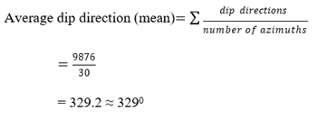
Table 7: showing grain size analysis data for sample 1
| Sieve Size (ɸ) | Mass Retained(G) | %Mass Retained | Cumulative % Retained |
| -2.25 | 6.05 | 1.21 | 1.21 |
| -1 | 35.85 | 7.17 | 8.38 |
| -0.24 | 115.65 | 23.13 | 31.51 |
| 0.23 | 63.85 | 12.77 | 44.28 |
| 0.74 | 60.75 | 12.15 | 56.43 |
| 1.23 | 59.95 | 11.99 | 68.42 |
| 1.74 | 51.95 | 10.39 | 78.81 |
| 2.74 | 79.25 | 15.85 | 94.66 |
| 3.74 | 20.75 | 4.15 | 98.81 |
| 3.74 | 2.25 | 0.45 | 99.26 |
| Pan | 3.7 | 0.74 | 100 |
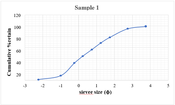
Fig. 9: Graph showing plot of sample 1
Table 8: Sample 1 statistical calculations for sieve analysis
| phi95 | phi84 | Phi75 | phi50 | phi25 | phi16 | phi15 | phi5 |
| 2.821928 | 2.067445 | 1.552984 | 0.470099 | -0.4539 | -0.74962 | -0.78248 | -1.58926 |
Sample two (2) collected from mining site opposite Njaba River
Table 9: Grain size analysis data for sample 2
| Sieve Size (ɸ) | Mass Retained(G) | %Mass Retained | Cumulative %Retained |
| -2.25 | 1.95 | 0.39 | 0.39 |
| -1 | 37.26 | 7.452 | 7.842 |
| -0.24 | 89.55 | 17.91 | 25.752 |
| 0.23 | 74.15 | 14.83 | 40.582 |
| 0.74 | 94.66 | 18.932 | 59.514 |
| 1.23 | 91.25 | 18.25 | 77.764 |
| 1.74 | 61.47 | 12.294 | 90.058 |
| 2.74 | 42.85 | 8.57 | 98.628 |
| 3.74 | 4.55 | 0.91 | 99.538 |
| 3.74 | 1.55 | 0.31 | 99.848 |
| Pan | 0.76 | 0.152 | 100 |
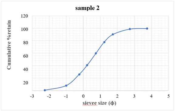
Fig. 10: Graph showing plot of sample 2
Table 10: Sample 1 statistical calculations for sieve analysis
| phi95 | phi84 | Phi75 | phi50 | phi25 | phi16 | phi15 | phi5 |
| 2.316663 | 1.488692 | 1.155788 | 0.483707 | -0.27191 | -0.65382 | -0.69625 | -1.47672 |
Sample nine (9) collected from gully site near Njaba River
Table 11: Grain size analysis data for sample 9
| Sieve Size (ɸ) | Mass Retained(G) | % Mass Retained | Cumulative % Retained |
| -2.25 | 0 | 0 | 0 |
| -1 | 0.8 | 0.151400454 | 0.151400454 |
| -0.24 | 15.5 | 2.9333838 | 3.084784254 |
| 0.23 | 36.6 | 6.92657078 | 10.01135503 |
| 0.74 | 72.6 | 13.73959122 | 23.75094625 |
| 1.23 | 102.6 | 19.41710825 | 43.1680545 |
| 1.74 | 100.6 | 19.03860712 | 62.20666162 |
| 2.74 | 118.1 | 22.35049205 | 84.55715367 |
| 3.74 | 30.4 | 5.75321726 | 90.31037093 |
| 3.74 | 30.3 | 5.734292203 | 96.04466313 |
| Pan | 20.9 | 3.955336866 | 100 |
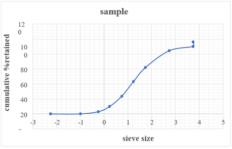
Fig. 11: Graph showing plot of sample 9
Table 12: Sample 9 statistical calculations for sieve analysis
| phi95 | phi84 | Phi75 | phi50 | phi25 | phi16 | phi15 | phi5 |
| 3.74 | 2.715072 | 2.312396 | 1.413012 | 0.77152 | 0.452293 | 0.415174 | -0.11004 |
Sample nine (8) collected from at Njaba River
Table 10: Grain size analysis data for sample 8
| Sieve Size (ɸ) | Mass Retained(G) | % Mass Retained | Cumulative % Retained |
| -2.25 | 0 | 0 | 0 |
| -1 | 1 | 0.520562207 | 0.520562207 |
| -0.24 | 2.66 | 1.384695471 | 1.905257678 |
| 0.23 | 3.6 | 1.874023946 | 3.779281624 |
| 0.74 | 9 | 4.685059865 | 8.464341489 |
| 1.23 | 20.8 | 10.82769391 | 19.2920354 |
| 1.74 | 26.9 | 14.00312337 | 33.29515877 |
| 2.74 | 81.23 | 42.28526809 | 75.58042686 |
| 3.74 | 37.76 | 19.65642894 | 95.2368558 |
| 3.74 | 8.5 | 4.424778761 | 99.66163457 |
| Pan | 0.65 | 0.338365435 | 100 |
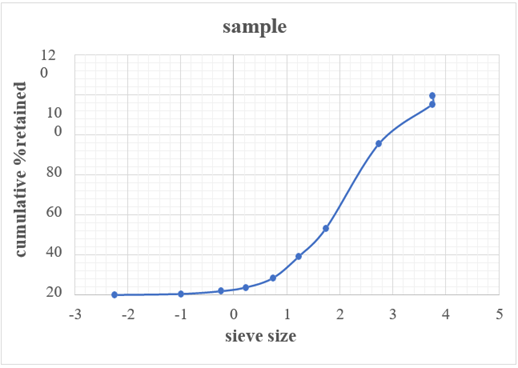
Fig. 12. Graph showing plot of sample 8
Table 14: Sample 8 statistical calculations for sieve analysis
| phi95 | phi84 | Phi75 | phi50 | phi25 | phi16 | phi15 | phi5 |
| 3.72795 | 3.168337 | 2.726274 | 2.135051 | 1.437887 | 1.081021 | 1.035767 | 0.362883 |