A Model on a Comparative Cross-Regime Analysis on Modelling and Forecasting of the Zimbabwe Stock Market Volatility Using ARCH (1), GARCH (1,1) and EGARCH (1,2) As the Extension to Account for Leverage Effects from April 2012 to April 2024

A Model on a Comparative Cross-Regime Analysis on Modelling and Forecasting of the Zimbabwe Stock Market Volatility Using ARCH (1), GARCH (1,1) and EGARCH (1,2) as the Extension to Account for Leverage Effects from April 2012 to April 2024

Brian Basvi

University of Zimbabwe

DOI: https://doi.org/10.51244/IJRSI.2024.1105047

Received: 15 May 2024; Accepted: 27 May 2024; Published: 12 June 2024

ABSTRACT

In order to account for the uncertainty underlying financial asset investments, volatility is crucial. Because of this, politicians, mutual fund managers, individual and institutional investors, and regulators of the financial industry are worried about volatility. In the context of the Zimbabwean stock market, this study aims to investigate how well three econometric models ARCH, GARCH, and EGARCH compare in terms of modelling and volatility predictions. The symmetry impact was estimated using the GARCH and ARCH models, while the asymmetric effect was captured by the EGARCH model, the third model. In light of this, this study employed daily averages for the mining and industrial indices over the period of 16 April 2012 to March 2024. This country was regarded in the literature for stock market volatility modelling and forecasting as efficient and having no volatility. The findings indicate that volatility persists, demonstrating that it takes time for the market to properly assimilate information into pricing and that shocks to conditional variance take longer to fade. Additionally, there is an asymmetry, which suggests that positive and negative news have distinct effects on the stock market and that positive news causes more volatility than negative news. Thus, we draw the conclusion that equally good and negative news have greater effects. During the epidemic, investors rely more on the good news to make wise judgments that increase their profits. Taking the outcomes into account, any measure meant to lessen the pandemic’s effects is beneficial for investment.

Keywords: ARCH, GARCH, EGARCH, Stylized facts, ZSE volatility forecasting.

List of abbreviations and acronyms

ARCH: Autoregressive Conditional Heteroscedasticity.

GARCH: General Autoregressive conditional Heteroscedasticity.

EGARCH: Exponential General Autoregressive Conditional Heteroscedasticity.

EMH: Efficient Market Hypothesis.

ZSE: Zimbabwean Stock Exchange

SECZ: Securities Exchange Commission of Zimbabwe.

INTRODUCTION

A statistical measure of the returns’ dispersion around the mean for a particular securities or market index is called volatility. Higher volatility indicates that a security’s value may be dispersed over a wider range of values, whereas lower volatility indicates that a security’s value fluctuates gradually rather than drastically. Crestmont (2021) measured the Standard & Poor 500 index’s volatility using daily averages, and then looked at the historical relationship between volatility and market performance. The study found that volatility and market performance have a statistically significant inverse connection, with volatility tending to rise in bear markets and decrease in bull markets.

Scholars, researchers, and others have focused a great deal of interest on modelling stock market volatility using high frequency data of financial time series in an effort to reduce investment risk. Financial time series have a leptokurtic distribution with fat tails and excess peaks near the mean. They are also characterized by volatility pooling or volatility clustering. Financial data series that exhibit clusters of high-volatility and low-volatility periods after one another are known as volatility pooling. Financial time series data, on the other hand, exhibit heteroscedasticity (variance that varies over time) and are dependent on past values (autoregressive) before perceived symmetric market information (conditional).

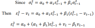
An ARCH model with conditional variance variation was proposed by Engle (1982). In the ARCH model, the conditional variance or restricted variance is dependent upon the squared error terms of the prior lags. Estimation and interception get harder the larger the lag squared error terms. A framework for creating volatility models and analysing stock market volatility was given by ARCH models. However, in order to address the issue of over parameterization, Taylor (1986) separately devised the GARCH model, a more frugal approach. The GARCH model’s prior squared errors and limited variances are what determine the conditional variance. The expansion of the AR to ARMA model is analogous to the extension of GARCH to ARCH. In the discipline of econometrics, the ARCH and GARCH models are frequently utilized, particularly for modelling volatility for financial time series. Numerous empirical applications of modelling conditional variance of financial time series have been made possible by the development of the ARCH and GARCH models.

The efficient market hypothesis theory (EMH) is generally accepted to hold that one cannot “beat the market.” Since stocks always trade at their fair market value, financial markets are likely very efficient in the sense that all information, both public and private, is completely reflected in stock prices, preventing monopolistic information from reaching investors (Chikoko, 2022). The Zimbabwe Stock Exchange (ZSE) was discovered to be weakly inefficient Mazviona (2016). According to Chipeta’s (2022) research, the Efficient Market Hypothesis (EMH) oversimplifies reality, as stock market returns are influenced by both positive and negative news. More complex models, such as exponential general autoregressive conditional heteroscedasticity (EGARCH), had to be developed because the ARCH–GARCH models could only simulate leptokurtosis and volatility pooling in a series. Nelson (1991) introduced the EGARCH, the logarithmic expression of conditional volatility that takes leverage effects into account.

The financial market’s memory for the past is longer than that of GARCH (1,1), according to (Guan, 2004). This has minimal effect on the model’s ability to predict future volatility. Evidence suggests that GARCH (1,1) outperformed EWMA (Exponentially Weighted) in terms of forecasting capacity. Evidence suggests that GARCH (1,1) outperformed EWMA (Exponentially Weighted Moving Average) in terms of forecasting power; however, they did not distinguish between the two. The time-varying conditional variance of a series was the stated target of all these models’ designs. Therefore, the current study attempts to simulate stock market volatility using several GARCH family models, including ARCH, GARCH and EGARCH models that account for leverage effects. This will allow for the provision of empirical evidence on the conditional volatility issue for the Zimbabwean stock market. The performance of the ZSE’s industrial index from April 2012 to March 2024 is shown in the graph below.

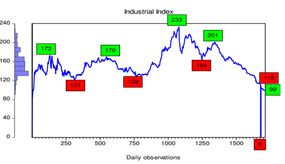
Fig 1: Industrial Index trend.

Conversely the mining index saw an increase of 5,26% to 1,60 points in the first quarter of 2024 after closing at 1,2 points in 2023. Nickel Corporation led the first day’s trading gains for the mining index, which measures the performance of the resource sector. The mining index’s performance on the ZSE from April 16 2012 to March 2024 is shown in the graph below.

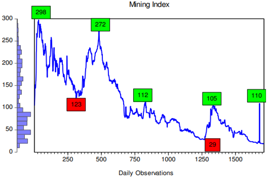
Fig 2: Mining Index trend

LITERATURE REVIEW

2.1 Volatility Definition and Measurement

In finance, volatility is often used to refer to standard deviation, σt , or variance, σ2. The simplest way of estimating volatility is taking daily squared returns from a set of observation as

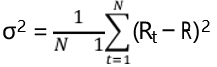
where  ̅R is the mean return.

The standard deviation statistic for the sample A distribution free parameter called σ根 stands for the sample’s second moment characteristic. It is only possible to determine the necessary probability density and cumulative density analytically when is connected to a standard distribution. But this approach provides erroneous volatility Taylor (1986). The closing price of an asset at the conclusion of a trading season is used to compute daily returns. The daily returns do not account for the price jumps that occur within a day. These spikes have the potential to be large and affect the volatility estimation.

Additionally, Stephen Figlewski (1997) pointed out that, particularly for small samples, the statistical characteristics of the sample mean make it a highly imprecise approximation of the true mean. According to Stephen Figlewski (1997), considering variations around zero rather than the sample mean usually boosts the accuracy of volatility predictions since the statistical characteristics of the sample mean make it an extremely inaccurate approximation of the true mean, especially for small samples. Models of volatility that were intended to take advantage of or lessen the impact of extremes were employed to estimate volatility. The square root is a biased estimate of Jensen’s inequality, but the equation above represents an unbiased estimate.

2.2 Volatility Models

Tsay (2005) postulated that it is well established that financial market volatility clusters before the market returns to a more stable environment where there is usually a period of extreme volatility. More precise and dependable volatility models can be constructed with the use of an autoregressive method. Engle first presented the ARCH model in 1982 (Engle, 1982). A number of the most widely used models for predicting market returns and volatility are the ARCH model and its extensions (GARCH, EGARCH, for example).

2.2.1 ARCH Model defined

The equation of the conditional mean:

The ARCH model also specifies conditional variance:

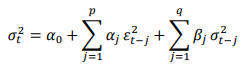
Generalized model ARCH (p):

If is low, then the conditional variance of the next period is small and alternatively if is high the conditional variance of the period is large Non-negativity constraint to ensure that

The derivation of unconditional variance:

For stationary ARCH requires

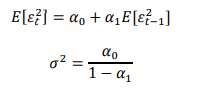
2.2.2 GARCH defined:

Derivation of the unconditional variance using the following definition

Unconditional variance

Generalized model GARCH (p,q)

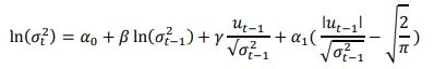
2.2.3 EGARCH defined:

The Exponential general autoregressive conditional heteroscedasticity (EGARCH) propounded by Nelson (1991) is one of popular models to account for leverage effects in stock returns.

2.3  Forecasting Volatility

Formally, forecasting volatility could be seen as findings that will minimize the error where an actual (or observed) volatility is over period t and f (.) is an error function. Below is a discussion of various error functions. It is possible to forecast volatility across various time intervals. One-day volatility, 10-day volatility, monthly volatility, and longer durations are the typical divisions. 10-day volatility is most frequently utilized in risk management, while daily volatility is typically employed to calculate risk metrics. Brooks (2008).

2.4  Empirical literature Review

Years later, Magnus (2012) study, which modelled stock market volatility of low income emerging stock markets in Africa for the Ghanaian stock market (1991–1996), Zimbabwe (1987–1995), and Nigeria (1984–1995), confirmed the findings of Ayadi’s (1998) study. Using the Freidman test, Ayadi (1998) also came to the conclusion that returns from the Ghanaian stock market are volatile. He discovered that there was no volatility in the Zimbabwean emerging stock market in the same investigation. But in a more recent study, Kamakar (2022) examined volatility in eleven low-income African nations using the EGARCH model. Additionally, Kamakar (2022) discovered that there was no volatility in the stock markets of Zimbabwe, Kenya, Egypt, Morocco, and Additionally, Kamakar (2022) discovered that the stock markets in Zimbabwe, Kenya, Egypt, Morocco, and Mauritius did not exhibit any volatility. While the stock markets in South Africa, Botswana, Swaziland, and the Ivory Coast were deemed to be inefficient, these markets were seen to be the most efficient in Africa.

Murekachiro (2021), modelling and forecasting the volatility of the Zimbabwean stock market years later, discovered a considerable divergence from normalcy and strong serial autocorrelation. When utilizing daily averages of the industrial index to anticipate volatility out-of-sample for the period of ten months, the asymmetric EGARCH (1,1) model performs better than the symmetric GARCH (1,1) model. When GARCH (1,1) and EGARCH (1,1) information criteria were applied, the findings indicated that EGARCH (1,1) was the most effective model for forecasting industrial index. Murekachiro (2022) kept quiet about the methodology used to determine returns during his investigation.

Nevertheless, GARCH (1,1) outperforms EGARCH (1,1) in other emerging market results. Gokcan (2020) revealed that the parsimonious GARCH (1,1) outperformed the complicated EGARCH (1,1) in modelling stock market volatility for seven emerging nations, including Malaysia and the Philippines. The optimal model for out-of-sample forecasting in the Malaysian and Filipino markets was later determined to be GARCH (1,1). Similar results were obtained by Xuii (2018) while modelling the Shanghai composite stock index between May 2000 and July 2010 indicating that GARCH (1,1) outperformed EGARCH and stochastic volatility models.

Using the KSE-100-time series, Kashif-ur-Rehman (2021) investigated the heavy tails, excess kurtosis, and volatility clustering. Using GARCH and ARCH, Kashif-ur-Rehman (2021) investigated the heavy tails, excess kurtosis, and volatility clustering of the KSE-100-time series. The purpose of this research was to compare the variance structures of data with high (daily) and low (weekly, monthly) frequencies. The results of this study indicate that the volatility clustering, which reflects the severity of shocks, was different for all the series by using the ARCH (1) and GARCH (1,1) models. The three return data series differed significantly in their statistical characteristics, as did the three series’ persistence of conditional volatility. When comparing the daily stock returns to other data sets, volatility clustering was more pronounced, indicating that the volatility models were responsive to the frequency of the data series. In another way, the findings showed that, in contrast to low frequency data series, the variance structure of high frequency data reflects the stylized facts associated with the volatility of stock returns, volatility clustering and a leptokurtic distribution with fat tails.

The results of Dawood (2021) for the Karachi stock exchange, where he discovered that the properties of the three data series are different from one another that is, the shocks occur on a daily basis and fade away within a month are also corroborated by the above study conducted on the KSE-100 index using ARCH and GARCH. Consequently, the daily industrial index and daily mining index data were employed in this study since daily data exhibits more volatile features than weekly, monthly, or annual data.

The jumps that cause the volatility patterns to alter for a respectable amount of time are associated with volatility clustering. These jumps, which tend to alter volatility patterns, won’t endure very long if a return series has a lengthy memory of its previous values. These jumps, which tend to alter volatility patterns, won’t persist for longer periods of time until the return returns to its typical level if a return series has a long memory for its past. The volatility clustering in return series was modelled by Maheu (2020) and the study’s findings showed that no shocks in the return series required a large amount of time to return to their normal level. At any particular period, the persistence of volatility is caused by a variety of factors that change from nation to nation. Global stock markets are typified by their persistent volatility. Global stock markets are typified by their persistent volatility. Batra (2021) discovered that the persistence of stock return volatility was growing as a result of financial liberalization in his analysis of the Indian stock market from 2010 to 2020.

Kauraa (2021) studied the impact of firm size and day of the week on volatility in her model of the stock market volatility from 2010 to 2020. The study’s findings provide proof that a company’s monthly volatility can range from low to high. Low volatility suggests low speculative positions, while high volatility indicates strong speculative ones. Penny stocks, or highly speculative stocks, are distinguished by their high return volatility in contrast to defensive stocks, which have lower return volatility.

Krugar (2017) examined the volatility of the Pakistani Karachi stock market, they discovered volatility clustering, a characteristic that is typical of emerging economies. The stock market’s inefficiency was indicated by the results, which showed that the GARCH model’s non-negative lagged returns significantly explained (current returns). Volatility clustering is the pattern whereby minor fluctuations in volatility were followed by smaller fluctuations and bigger fluctuations in volatility were followed by larger variations.

Gushan (2022) research, the GARCH (1,1) model overvalues new observations at the expense of older observations. Because extreme observations have less of an effect on projections when absolute deviations of returns from the mean are employed, GARCH (1,1) is a good model for forecasting. Because they are not over parameterized, more complex models like GARCH (1,1) perform best on in-sample forecasts. Over parameterized models, on the other hand, include factors that raise the possibility of estimate error but consistently perform worse on out-of-sample forecasts.

Floros (2022) used asymmetric models to study the volatility using daily data from two Middle Eastern stock indices. The leverage impact was evident from the EGARCH model’s parameter estimations, which for both indices revealed a negative and significant value. Weak transitory leverage effects were observed in the conditional variances of the asymmetric GARCH model, and the study provides evidence that higher risk does not always equate to higher returns.

EGARCH is the most effective model among the other asymmetric family of GARCH models for evaluating stock market volatility (Ahmed, 2021). A sample of data that was collected between 2015 and 2023 and showed a considerable divergence from normalcy was used in the study.

Sweyn (2022) used the symmetric GARCH model, E-GARCH, and GARCH in mean (GARCH-M) to study daily and monthly returns on the Colombo Stock Exchange (CSE). It was discovered that EGARCH (1,1) was the most suitable model for simulating how news affects Sri Lankan.

The study conducted by Garikai (2023) examined the relationship between news and stock market volatility in India, as well as the potential impact of leverage effects on Indian stock prices using data spanning from 2012 to 2022. The findings indicated that power garch (PGARCH) was the most effective asymmetric model, while GARCH (1,1) was the most suitable symmetric model. The GARCH (1,1) was found to be statistically adequate in capturing the symmetric effect.

Wellington Mazviona (2022) carried a study on EGARCH for leverage effects in their study day of the week effect on stock returns. These studies attempted to model the volatility of the Zimbabwean stock market. To choose the best model for volatility estimates and forecasting on the ZSE, the current study used symmetric ARCH, GARCH, and EGARCH models to account for leverage effects on stock returns.

METHODOLOGY

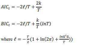
The study applied three different models to model and anticipate the volatility of the Zimbabwean stock market: exponential autoregressive conditional heteroscedasticity (EGARCH (1,2)), general autoregressive conditional heteroscedasticity (GARCH (1,1)) and autoregressive conditional heteroscedasticity (ARCH (2)). The variance equation and the mean equation are two separate equations that are estimated using the Eviews-7 program which is also used for data analysis and model estimation. The Bayesian Information Criterion (BIC) and the Akaike Information Criterion (AIC) are the two most often used techniques for selecting models. While the Bayesian Information Criteria penalizes more complex models (those with many parameters) relative to simpler models, the Akaike Information Criteria fundamentally incorporates the idea of cross validation, but only in a more theoretical sense. Consequently, the model with the lowest AIC and BIC value ought to be selected when comparing the AIC and BIC values of two or more models. Eviews formulates the test statistic from a log- likelihood function using maximum likelihood estimation algorithms. Eviews equations are

3.1  Testing for Stationarity

Since stock returns are typically described as nonstationary, it is impossible to determine in practice whether a series is stationary at first difference I (1) or first level I (0). The most basic test for stationarity in stock returns is the Dickey Fuller (1979) Augmented Dickey-Fuller. The testing process, given an econometric model, is as follows:

The hypothesis to be tested is:

To obtain the test statistic regress yt on yt 1 that is the lagged values of yt to test for stationarity at first level I(0) or alternatively regress the first difference I(1) which is given by following equation . The test statistic is the usual t-ratio given by:

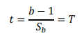
where sb is the standard error of “b” from the regression’s. n The null hypothesis H0 is rejected in favour of H1 if the series is stationary.

3.2 Testing for Heteroscedasticity and Serial autocorrelation

The Engle’s ARCH test, which is typically performed on raw data with the user-specified number of lags “p,” is used to test for heteroscedasticity. The first step is to estimate the mean equation and test for ARCH effects in the residuals. If the data is sampled daily instead of at a low frequency, this test will yield more accurate findings, other things being equal. Another name for the test is the autocorrelation in the squared residuals test. For each of the q lags of the squared residuals, a joint null hypothesis is tested to see if the values of the coefficients are all substantially different from zero. Reject the null hypothesis if the test statistic’s value is higher than the distribution’s critical value.

3.3  Autocorrelation function and Partial auto-correlation Function

The dependence in the data is ascertained by computing correlations for data values at varying time lags. This is done by plotting the sample autocorrelation function (ACF):

And  ̅y is the sample mean. For every time lag separation, the autocorrelation should be close to zero if the series is the result of a totally random occurrence. If not, there will be a large non-zero autocorrelation in one or more variables. Analyzing serial dependencies using the Partial Autocorrelation Function (PCF) is another helpful technique. Similar to the autocorrelation function, the partial autocorrelation function is calculated by eliminating the autocorrelation with all of the lag’s elements.

3.4  Testing for Forecasting power

 Models with the lowest error measure would be deemed to be the most accurate when the mean squared error (MSE) or mean absolute error (MAE) from one model was compared to those from other models estimated using the same data and prediction period. Brooks (2008). To compare the calculated models’ forecasting power, the U-statistic is also employed., For  , this implies that the forecasting technique is as good as guessing and if   , it means that the forecasting technique is worse than guessing. Therefore, it is always desirable for the U-statistic to be close to zero and less than 1. The closer the Theil U-statistic is to zero, the more efficient the model becomes in producing accurate forecasting results.

RESULTS

Appendix I contains the distributional features of the mining index and industrial index, which were computed and reported. The distribution of the industrial index is positively skewed, as indicated by the average industrial return of 0.1361890, excess kurtosis of 1569.724, and skewness of 38.78326. The latter indicates the degree of deviation from normalcy. According to the Jarque-Bera statistics, the mining and industrial indices do not follow a normal distribution, and at the 1% level of significance, we can accept or reject this conclusion. On the other hand, every descriptive statistic displayed for the mining and industrial index demonstrates proof of the stylized facts about stock market prices, which include large skewness and leptokurtosis.

4.1  Testing for Stationarity:

The mining and industrial indices’ stationarity has been tested using enhanced Dickey Fuller. Tables 1 and 2 below present the findings of the ADF test for the mining index and the industrial index, which indicate that both return series are stationary at level I (0):

Table 1: Industrial Index

Period			Industrial index series Critical values
	ADF statistics	1%	5%	10%
2012-2024	-28.46031	-3.433982	-2.863031                        -2.567611

Table 2: Mining Index

Period	ADF ststistics		Mining index series critical values 5%                        10%
		1%
2012-2024	-38.08755	-3.433973	-2.863027       -2.567609

ADF test includes intercept without trend.

4.2  Testing for Heteroscedasticity and autocorrelation

The heteroscedasticity test was employed for both the mining and industrial indexes to check for GARCH and ARCH effects. The residuals acquired by estimating the ordinary least squares regression of the mean equation an autoregressive moving average are used to assess the ARCH and GARCH effects. In order to reject and conclude in favour of the presence of GARCH effects, the joint null hypothesis test for the coefficients of squared residuals computed at q-lags only needs one coefficient to be statistically significant from zero. The residuals of the calculated conditional mean equation, which were an ARMA (1,2) and ARMA (1,1) for the mining index and industrial index with 5-lags, respectively, were found to contain the GARCH and ARCH effects. Appendices III and IV provide the findings from the testing of heteroscedasticity on the mining and industrial indexes.

4.3  Autocorrelation function (ACF) and Partial Autocorrelation function (PACF):

The existence of ARCH and GARCH effects is further supported by the correlogram plot of the squared errors derived from the estimated ARMA (1,2) and ARM (1,1) for the mining index and industrial index, respectively. It is implied that the squared errors are autocorrelated with the squared errors of the previous period by the autocorrelation function (ACF) and partial autocorrelation function (PACF) spikes, which are beyond limits.

4.4  Presentation of results:

The Ordinary Least Squares (OLS) model of ZSE stock market volatility is consistent but inefficient due to the existence of both GARCH and ARCH effects in the time series data for the mining and industrial index. In order to account for the ARCH and GARCH structure, ARCH, GARCH, and EGARCH were used. generated findings with parameters that were statistically insignificant; as a result, we estimated high order ARCH (2) for industrial return series. Below is a presentation of the estimated models:

4.4.1  Estimated ARCH model:

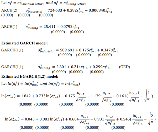
ARCH(2)rindustrial estimation

For periods (t-1) and (t-2), the ARCH (2) model yielded substantial coefficient of the squared residuals; nevertheless, the results did not meet the non-negativity requirement needed to estimate the Autoregressive conditional heteroscedasticity model. Because of the non-negativity criterion, (conditional variance),

Remedial action to this problem is to estimate popular GARCH (1,1).

ARCH(1)rmining

The coefficients have a highly statistically significant sign and are for the predicted autoregressive conditional heteroscedasticity of order p=1. This indicates a substantial determination of conditional variance by the squared residual for (t-1). Because the ARCH (1) coefficients are statistically significant starting at zero, the model can accurately represent the ARCH structure in the mining return series. As a stand-in for risk measurement, conditional variance indicates that return increases with increased volatility. The model has correctly modelled the arch structure in the industrial return series, according to the test for ARCH effects conducted after model ARCH (2) rind was estimated.

GARCH(1, 1)rindustrial

The findings in Appendix VIII demonstrate that the industrial return series’ volatility clustering can be adequately captured by GARCH (1,1). The coefficients derived from GARCH (1,1) estimation, constant (ao), ARCH term (a1), and the GARCH term (β) have strong form statistical significance with predicted signs. The impact of the squared error term (εt2<΀1) and the lag conditional variance (σt2~΀2) on the present conditional variance (σ) t(2) is demonstrated by the relevance of the ARCH and GARCH terms. A stationary GARCH is indicated by the combined value of the ARCH term and GARCH term (a1 + β = 0.0472), which is less than 1. This suggests that ZSE has been in a state of protracted serenity where tiny changes are followed for a long time by small changes.

GARCH(1, 1)Tmining

For the sake of modelling and forecasting Zimbabwe stock market volatility using univariate GARCH(1,1), we assumed a normal distribution of conditional mining returns. Although the GARCH parameter in the GARCH(1, 1)Tmin estimation result was negative, the coefficients in the output were statistically significant. GARCH(1,1) under generalized error distribution (GED) was computed however in order to accurately describe excess kurtosis in the mining returns. A specific instance of the Gaussian distribution is the GED distribution which has wider tails. The sum of ARCH and GARCH parameter (a1 + β = 0.513) which is less than 1, meaning GARCH(1,1)Tmin is a stationary GARCH.

EGARCH(1, 2)TindustTial

It is claimed that fluctuations in volatility have a negative correlation with stock prices. Munk (2013), Claus. To address this issue, EGARCH was developed. Since the conditional variance is always positive according to the EGARCH given as the logarithm of the conditional variance, the model parameters are unrestricted. The impact of positive or negative news on stock returns is determined by the leverage factors, Y1 and Y2. Take advantage of the positive news effect

, for bad news . Results presented in appendix XI clearly indicate that Y1and Y2

are negative and significant which is evidence of asymmetry structure in the industrial returns. The news impact curve illustrates the additive effects of bad news, which is that it affects the movement of industrial returns and causes a greater present conditional variance than good news.

EGARCH(1, 2)Tmining

The leverage parameters Y1 = 0.604and Y2 = 一0.931are statically different from zero or strongly significant. The parameter Y1 has positive effect to next period‟s conditional variance and Y2 has negative effect, but however the additive effect is positive as shown in figure 8. The positive section of the news impact curve is larger than the negative section.If a shock occurs on a return series, ln(σ ) respond asymmetrically  if at21  = 0.  If the negative and positive extreme points are eliminated, the news effect curve for EGARCH on mining returns indicates that the shocks to the mining return series are nearly symmetrically distributed.

4.5  Model diagnosis:

In order to determine whether the family of ARCH and GARCH models has been successful in capturing volatility pooling in the industrial and mining returns, post-estimation testing for ARCH and GARCH effects is carried out in this section. Model diagnosis is carried out by analyzing the residuals of the fitted models. The results reported in appendix XIII with F-statistic (0.7878) and P-values (0.7877) for GARCH(1, 1)Tind show there is no evidence of ARCH effects at 5% level of significance, so we reject H1 and come to the conclusion that there are no ARCH/GARCH effects. The results of assessing the ARCH effects for the model ARCH (1) Tmin are also shown in Appendix XII. The F-statistic (0.6133) and P-value (0.6130) are both statistically not different from zero, leading us to infer that there are no ARCH effects. Since the ARCH LM test verified that there were no GARCH or ARCH effects in the squared residuals of the fitted models, we can therefore draw the conclusion that there is no serial autocorrelation.

The fitted residuals for all estimated models’ normality tests revealed that their distributions resembled those of normal distributions, indicating that the models’ specifications were accurate and sufficient to capture leptokurtosis and volatility clustering in mining and industrial return series.

4.5.1  Testing for goodness of fit:

R-Sqiuared statistic is used test for goodness of fit. The estimation procedures used in this research are that of the GARCH type therefore we expected R2 to be negative and low for all models estimated. The reason is because ARCH and GARCH models assume perfect fit for the conditional variance equation (note that conditional variance equation for GARCH or ARCH models has no error term). The results confirmed the theory of ARCH and GARCH modelling in terms of magnitude and expected sign for R2 .

Model selection criterion: The best final model that made it through the model diagnosis step was chosen using the model selection criteria. Among all the models employed to model volatility for industrial return series, the model with the highest efficiency was identified using the Akaike information criteria and Schwarz information criterion (SIC). According to the information in the first portion of the table, GARCH(1,1) has the lowest index value for both the Schwarz and Akaike information criteria. All of the models used to model mining return series are shown in Table 3’s second part. The most effective model, GARCH(1,1), has the lowest values for the Akaike and Schwarz information criteria. EGARCH(1,2) exponential autoregressive conditional heteroscedasticity models were shown to be the second best model for describing the excess kurtosis and volatility of the Zimbabwean stock market.

Table 3: Summary of estimated models

Model estimated	AIC	SIC
GARCH(1,1)rindustrial	9.179434*	9.192163*
EGARCH(1,2)rindustrial	9.376864**	9.395958**
ARCH(1)rmining	6.104927***	6.114474***
GARCH(1,1)rmining	4.589948*	4.605859*
EGARCH(1,2)rmining	5.526130**	5.545223**

Note: *and ** indicate model with the lowest AIC and SIC index value. ARCH(2)rindviolated the non-negativity constraints therefore it was left in analysis of results.

4.5.2  Forecasting Evaluation:

This section looks at each fitted model in the study’s out-of-sample forecasting capability. Mean Absolute Error (MAE) and Root Mean Square (RSE) are two symmetric loss functions that were employed. An additional measure for evaluating the forecasting power of fitted models of the ARCH and GARCH types was Theil’s U- statistic.

Table 4: Summary for out-of sample forecasting results

Model estimated	RME	MAE	Theil‟s U-Statistic
GARCH(1,1)rindustrial	32.22173*	2.096519*	0.980455
EGARCH(1,2)rindustrial	32.24581**	2.652606**	0.961090
ARCH(1)rmining	6.404081***	1.901505***	0.993811
GARCH(1,1)rmining	6.404570*	1.889434*	0.999994
EGARCH(1,2)rmining	6.403821**	1.926026**	0.982125

Note: *and ** indicate model with the lowest MAE and RME index value.

The forecasting findings provided in appendix XIV, which support GARCH(1,1)rind as the best model for forecasting industrial returns on the Zimbabwe stock market, are summarized in the statistics (RME and MAE) presented in table 3 above. The model’s forecasting outcomes are superior to guesswork when the Theil’s U- statistic is less than 1. is the most effective out-of-sample forecasting model for mining returns when taking into account the Mean Absolute Error statistics shown in Table 3. For returns series, there is no significant difference between the RME and Theil’s U-statistic (differentiated by ± 0.001). The second-best model for predicting mining returns in the Zimbabwe stock market is ARCH(1). In terms of predicting mining and industrial returns, In terms of predicting mining and industrial returns, EGARCH(1,2) has not done well. Since the Theil’s U-statistic for each fitted model is less than 1, we can fairly say that any of the fitted models mentioned above can be utilized for forecasting. The remaining forecasting findings are detailed in appendices XIV (a) through XIV (e).

DISCUSSION OF RESULTS

The results illustrates how far the mining and industrial returns deviate from the 45-degree line, indicating excess kurtosis and volatility clustering. The industrial and mining return series exhibit non-normality as indicated by the large maximum and lowest values in the histogram plots where the mean and median values are nearly zero. Additionally, price and return fluctuations are clearly shown in this. Both the mining return (16226020) and the industrial return (1.75e+08) have strong Jargue-Bera statistics with (0.000) p-values, indicating that both series have fat-tailed distributions. This further supports the ARCH and GARCH processes in the returns series. The findings of this study’s normalcy test support the findings of Ahmed (2021) investigation. Figures 5 and 6’s squared residual correlogram plots demonstrate that the mining and industrial return series are white noise processes with ACF and PACF spikes that are larger than expected for the first and second lags, indicating the presence of GARCH and ARCH effects in the daily data. The results presented demonstrate that the mining and industrial returns series have highly skewed and leptokurtic distributions, yielding findings akin to those of Kashif-ur-Rehman (2021). Maheuy (2020) came to the same conclusion: random walk processes with time- varying properties are what drive stock market returns.

4.6.1   Industrial returns series:

Evaluating in-sample fit the Akaike information criteria and Schwarz Information criteria was used. GARCH(1,1)Tind has the lowest AIC (9.179434) and SIC (9.192163) index value for modelling industrial returns as shown by the summary of results in table 3 in the previous chapter (or in appendix VIII). EGARCH(1,2)Tind has relatively high AIC (9.376864) and SIC (9.395958). The GARCH(1,1) clearly outperforms EGARCH(1,2) in modelling volatility clustering and excess kurtosis.

The evaluation of out-of-sample forecasting was conducted using the Mean Absolute Error (MAE), Root Mean Error (RME), and Theil’s U-statistic with summary data provided. Two loss functions, RME and MAE, backed GARCH(1,1)Tind as the best forecasting model,surpassing EGARCH(1,2)Tind. Both models’ Theil’s U-statistics are smaller than 1, indicating that their forecasting accuracy outperforms conjecture. Similar findings were reported by Gokcan (2000) and Chaung et al. (2007), who came to the conclusion that the GARCH(1,1) model performs better than the EGARCH model.

4.6.2   Mining returns series:

Despite the ARCH parameter not being very near to 1, the results shown in Appendix VII demonstrate that the coefficients of ARCH(1)rmin are statistically significant and positive. This indicates that the mean reversion of conditional variance provides evidence of a long memory to the past in the mining return series. The outcomes have resemblance to Pryymachenko’s (2003) research on the Ukrainian stock market. The results for GARCH(1,1) and EGARCH(1,2) are also displayed in Appendices IX and XI, with all parameters being statistically significant and showing the predicted indications.

However, GARCH(1,1)Tmin for a generalized error distribution (GED) has the lowest AIC (4.589948) and SIC (4.605859) than ARCH(1)Tmin with AIC = 6.104927, SIC= 6.114474 and EGARCH(1,2)Tminwith AIC= 5.526130, SIC = 5.545223. All statistics presented in table 3 indicate that GARCH(1,1)rmin is the most appropriate model in modeling ZSE stock market volatility. The study’s findings support Wennstrom’s (2014) conclusion that the GARCH(1,1) model is superior to the ARCH(p). The second-best model is EGARCH(1,2)rmin. Table 4 also displays summary data for out-of-sample forecasting evaluation across all models suggested for mining return forecasting. With 0.001 acting as the differentiating factor, the RME and Theil’s U-statistics for each of the three models do not differ from one another statistically. The Mean Absolute Error revealed GARCH(1,1)rmin as the best in-sample fit (fitted model) and forecasting model clearly outperforming EGARCH(1,1)rmin and ARCH(1)rmin. Xu (1999) found similar results that GARCH model was superior to EGARCH,GJR-GARCH and Stochastic Volatility (SV) models.

CONCLUSION

Research on modeling and forecasting financial time series volatility has grown increasingly fruitful (Ahmed and Suliman, 2011). Any increase in market volatility typically results in calls from the public for government regulators, as volatility in speculative markets is perceived by the public as a valid worry (Shiller, 2006). After determining if ARCH effects were present, the study was able to investigate the volatility of the Zimbabwean stock market using both symmetric and asymmetric models. The ARCH (1,1), GARCH (1,1), and EGARCH (1,1) models were all calculated in the study. The identification, estimating, and checking phases of the model- building technique have been investigated and put to use. We developed and examined the time series ARCH and GARCH in this study.

We developed and examined the times series ARCH, GARCH, and EGARCH models in this study. The ARCH family of models essentially presupposes that the data to be modelled must be heteroscedastic, that all parameters in the variance equation must be positive (to ensure non-negativity condition for the conditional variance), and that the current conditional variance is dependent upon the prior observations and conditional variance. The Tindust returns series is best fitted by a GARCH(1, 1) model with a t-distribution, and the Tindust returns series is best fitted by a GARCH(1, 1) model with a GED distribution, according to minimal AIC values. The study’s findings suggest that for the stock market to thrive, favorable conditions for investments, including macroeconomic stability, must exist. For investors to make wise investment decisions, the future must be predictable. The economy need policies aimed at lowering stock market volatility.Policy makers and investors can both benefit from the empirical findings. Compared to the mining industry, the industrial sector’s stock market is more volatile. In the case of leverage effects, the null hypothesis was accepted. Therefore, although GARCH(1,1) is utilized to model and forecast the volatility of the Zimbabwean stock market, EGARCH(1,2) should be used as a supporting tool in assessing the impact of leverage effects in stock price movement.

The study suggests that investors, brokers, and portfolio managers use daily data (high frequency data) to model and forecast Zimbabwean stock market volatility based on the empirical results gained. The explanation is that, as these properties are clearly observable in high frequency data, the returns on the Zimbabwean stock market showed characteristics of a highly volatile market that are volatility clustering.

REFERENCES

1. Ahmed, M., and A. E. Aa l. 2011. „Modelling and Forecasting Time Varying Stock Return Volatility in the Egyptian Stock ‟ International Research Journal of Finance and Economics 78:96– 113.
2. Ayadi. F.O, Dufrene U.B, and Chatterjee. A, (1998). Stock returns seasonalities in low-income African emerging markets. Managerial Finance, Vol. 24, No. 3, pp. 22-32
3. Batra, A (2004), “Stock Return Volatility Patterns in India,” Indian Council for Research on International Economic Relations, Working Paper 124.
4. Bekaert. G and Wu. G, 2000, Asymmetric volatility and risk in equity markets. The review of financial studies, vol, 13, 1.
5. Bollerslev, 1986. “Generalized   Autoregressive Conditional  Heteroskedasticity”, Journal of Econometrics 31 (3): 307–27.
6. Bollerslev,T.1986.„Generalized Autoregressive Conditional ‟Journal of Econometrics 31 (3): 307–27.
7. Bonga G, 2014, “Empirical Analysis of Stock Returns and Volatility of the Zimbabwean Stock Markets”, Volume 5, Issue 6. Ver. III (Nov. -Dec. 2014), PP 46-57.
8. Brooks, (2008). Introductory Econometrics for Finance, Cambridge Univ. Press, 2nd Edition.
9. Caiado. J (2004), “Modelling and forecasting the volatility of the Portuguese stock index PSI-20,” Munich Personal RePEc Archive (MPRA) Paper No. 2304, posted 2007.
10. Chikoko and W. Muparuri 2013, Zimbabwe Stock Exchange and Efficiency in the Multiple Currency Exchange Rate Regime, Journal of Business and Economic Management, 1(3) , 41-47.
11. Chowa T., Nyanhete A.I., and Mhlanga R. 2014. An Event Study Of The Zimbabwe Stock Exchange (ZSE): Implications For Post-dollarisation Market Efficiency. Mediterranean Journal of Social Sciences, Vol 5 No 3.
12. Crestmont Research, “Beyond the Horizon 2011”. [Online] available at Inve stopedia.com [Accessed 12 April 2016].
13. Dawood. M (2007), “Macro Economic Uncertainty of 1990s and Volatility at Karachi Stock Exchange”, Munich Personal RePEc Archive (MPRA) Paper No. 3219, posted, 2007.
14. Ederington L. and Guan W, 2004. “Measuring Historical Volatility, Journal of Futures Markets, pp. 2-
15. Ederington L.H and Guan. W 2004, Measuring Historical Volatility, University of South Florida St.
16. Engle, R. 1982. „Autoregressive Conditional Heteroskedasticity with Estimates of the Variance of uk Inflation.‟ Econometrica 50 (4): 987– 1007.
17. Figlewski. S, 1997, Forecasting volatility, Financial Markets, Institutions, and Instruments 6, Blackwell Publishers: Boston.
18. Floros, C (2008), “Modelling Volatility using GARCH Models: Evidence from Egypt and Israel,” Middle Eastern Econ., ISSN: 1450-2889 Issue 2.
19. Gokcan, C (2000). Techniques for verifying the accuracy of risk measurement models. Finance and Economics Discussion Series 95-24, Board of Governors of the Federal Reserve System (U.S.).
20. Hassan MK, Islam AM, Basher (2000). “Market Efficiency, Time-Varying Volatility and Equity Returns in Bangladesh Stock Market.” Working Paper, Department of Finance and Economics, University of New Orleans.
21. Jegajeevana S, “Return Volatility and Asymmetric News Effect in Sri Lankan Stock Market”, Economic Research Department Central Bank of Sri
22. Kamakar.  Y (2006). “Recovering Risk Aversion from Option Prices and Realized Returns,” Review of Financial Studies, 13, 433–451.
23. Kaura, H (2002). Stock Market Volatility in India, New Delhi:Deep & Deep
24. Li J (2007). “Three Essays on Modeling Stock Returns: Empirical Analysis of the Residual Distribution, Risk-Return Relation, and Stock-Bond Dynamic ” Unpublished Ph. D Thesis.
25. Magnus J and Fosu O. E, 2006, Modelling and Forecasting Volatility of Returns on the Ghana Stock Exchange using Garch Models, American Journal of Applied Sciences 3 (10): 2042-2048.
26. Maheuy, H. McCurdyz (2003). “News Arrival, Jump Dynamics and Volatility Components for Individual Stock Returns.” Unpublished Research Paper.
27. Mazviona W and Nyangara D, A Test of the Weak Form Efficiency of the Zimbabwe Stock Exchange after Currency Reform, International Journal of Business, Economics and Law, 2(2), (2013), 43-48.
28. Mazviona B.W and Ndlovu M.W, Day of the week effect on the Zimbabwe Stock Exchange: A non-linear GARCH analysis, 3(3), (2015).
29. Mazviona. W. and Nyangara D, 2013. A Test of the Weak Form Efficiency of the Zimbabwe Stock Exchange after Currency Reform, International Journal of Business, Economics and Law, 2(2), 43-48.
30. Mbululu, and Chipeta C, 2012. Day of the Week Effect: Evidence from nine Economic Sectors on the JSE, Investment Analysts Journal, 41(75), 55-65.
31. Mittal, A. K., D. D. Arora, and N. Garikai. 2012. „Modelling the Volatility of Indian Stock Market.‟ gitam Journal of Management 10 (1): 224–43.
32. Murekachiro. D, “Time Series Volatility Forecasting of the Zimbabwe Stock Exchange”, The International Journal Of Business & Management (ISSN 2321–8916).
33. Nelson, D, 1991. “Conditional Heteroscedasticity in Asset Returns: A New Approach”. Econometrica 59 (2): 347–70
34. Pryymachenko, I 2003, Stock Price Volatility and its determinants on the emerging Financial Market of Ukraine, National University of Kyiv-Mohyla
35. Rafique. A and Kashif-ur-Rehman, 2011. Comparing the persistency of different frequencies of stock returns volatility in emerging market: A case study of Pakistan, African Journal of Business Management, 5:59-67.
36. Rajanikanth .C, Lokanadha Reddy. E, Jyothsna. C 2016, “Stock Market: Analysis of Volatility and its Impact on Investors in choosing Securities for Investment”, 4, No. 1, April 2016.
37. Rizwan M.R and Krugar. S.U 2007, “ Stock Return Volatility in Emerging Equity Market (KSE): The Relative Effects of Country and Global Factors”, 3 No.2 June 2007, Pp. 362 – 375.
38. Shamiri, A. and Z. Isa (2009). Modeling and forecasting volatility of Malaysian stock markets. Journal of Mathematics and Statistics, 3, 234-240
39. Thomas, S (1995). “Heteroscedasticity Models on the Bombay Stock ” Working Paper, University of Southern California, Department of Economi