Application of Copula Methods in Financial Risk Management: Case of the Zimbabwe Stock Exchange and the Victoria Falls Stock Exchange.

Application of Copula Methods in Financial Risk Management: Case of the Zimbabwe Stock Exchange and the Victoria Falls Stock Exchange.

Brian Basvi

University of Zimbabwe

DOI: https://doi.org/10.51244/IJRSI.2024.1105042

Received: 15 May 2024; Accepted: 27 May 2024; Published: 11 June 2024

ABSTRACT

In order to minimize risks and create a safe investing environment, financial risk management is becoming more and more crucial for individuals, financial organizations, and even entire nations. Accurately assessing financial risks and using that information to inform wise investment choices can give an investor a competitive edge as well as significant returns. In actuality, real-world financial variables limit the ability to estimate financial risks. On the other hand, a wealth of data indicates that financial variables typically have asymmetric dependency, skewness, and fat tails. In three ways, the conventional approaches to financial risk management based on normally distributed hypotheses are put to the test by these stylized characteristics of financial variables. First, the univariate normal distribution or other elliptical distributions are unable to adequately fit the distribution of the univariate variable. Second, despite their straightforward tractability, multivariate variables’ extra kurtosis and skewness are not captured by their normal distribution. As a result, the dependence risks associated with multivariate financial variables may be underestimated. Finally, when the joint distribution of various variables is non-elliptical, linear correlation which is typically employed to characterize the dependence of various variables in traditional portfolio risk management is likewise insufficient. This research uses a promising technique based on copulas in conjunction with GARCH and realized volatility models to examine the risks associated with multivariate financial variables in order to address these issues. The multivariate distributions are constructed using copulas in conjunction with GARCH and Realized Volatility models which are then utilized to evaluate portfolio risks in financial market. The findings demonstrate that copula-based models outperform conventional models in fitting financial data. Second, a variety of marginal models have a notable impact on the value at risk of the portfolio, including the GARCH and realized volatility models. Lastly, both the dependence structure and the marginal distribution exhibit notable skewness. Consequently, compared to the normal or Student-t distribution, the skewed Student-t distribution fits some datasets better.

Key Terms: Copulas, Value at Risk, Financial Risk Management, viability and profitability

INTRODUCTION

Over the past few decades, financial risk management has gained popularity and significance as a concept that focuses on ways to use financial instruments to hedging risk exposure. A number of factors have contributed to the emergence of financial risk management as a discipline, including the exponential growth in trading activity since the late 1960s, the massive increases in the variety of instruments traded in the markets, and so on. The rapid growth in trading activity and instrument types has occurred in an environment that is frequently volatile, which exposes firms to higher levels of financial risk that is, the possibility of financial gain or loss due to unanticipated changes in underlying risk factors risk management (Dowd, 2023). The measurement of one specific type of financial risk market risk, or more specifically, equity risk is the focus of this paper.

Financial risk is something that anybody involved in investing, be it an individual, a financial institution, or a corporation. Investors can only make money while making prudent financial risk management decisions; otherwise, their investments could result in losses rather than gains. Due to inadequate risk management, many organisations failed due to bankruptcy. This includes the Royal Bank which faced liquidity changes in 2012, Trust bank in which the license was revoked in 2017, Interfin Bank, Genesis Investment, Renaissance Merchant bank failed due to improper financial risk management practices. As a result, investors should actively plan for the ramifications of unfavourable results, employ effective risk management techniques to reduce their exposure to risk, and generally improve their readiness for the unavoidable uncertainty (Mazambara, 2022). The main issue in finance risk quantification is the main issue with financial risk management. The Value at Risk (VaR) model is one of the most popular risk measurements and has evolved into a standard for aggregating hazards across several elements. Several risk measuring techniques have been developed in the past. VaR, which was created in reaction to the early 1990s spike in financial market volatility, is being utilized by both financial and non-financial organizations more and more.

This risk measure’s enormous popularity is mostly because to its straight forward conceptualization, simplicity in computation, and immediate application. Value at Risk (VaR), which is easily employed by banks, brokerage firms, investment funds, and even non-financial entities, reduces the (market) risk associated with any portfolio to simply one monetary value, i.e. the loss linked to a certain likelihood. Nonetheless, condensing a large number of complicated and undesirable results into a single figure inevitably entails some trade-off between the demands of many consumers (Engle,2020).

LITERATURE REVIEW

The joint multivariate distribution and copula

It is necessary to understand the relationship between these variables when modelling the multivariate variables. Because linear correlation, also known as Pearson’s correlation, is typically easy to compute and has the naturalness as a measure of dependency in multivariate normal distribution, which is typically utilized in theory and practice, it is traditionally used to explain the link between variables. Nonetheless, the existing body of financial research has extensively documented instances of non-normality. As a result, when normality is altered, the dependency between variables is not well described by linear correlation. As a result, stronger substitute correlations are suggested, including rank correlation, which is invariant under monotonic transformations and in the sense of perfect dependency. Examples of these correlations are Kendall’s rank correlation and Spearman’s rank correlation. However, in contrast to linear correlations, they are not moment-based correlations and do not lend themselves to the same sophisticated variance-covariance manipulations.

The copula is designed to flexibly describe the relationship between variables. A useful and effective technique for describing dependent risks is the copula function. It divides a multivariate vector’s joint distribution into its boundaries and dependencies. The copula idea has advanced quickly in the last many years. Sklar (1959) first proposed this, demonstrating that any n-dimensional joint distribution function could be broken down into its n marginal distributions, which fully describe the shape, location, and scale parameters of the n variables (i.e., skewness, kurtosis, mean, and standard deviation), and a copula, which fully describes the dependence between the n variables n variables, and proves the well-known. Embrechts et al. (1999) introduced this concept to the finance literature. Copulas have already been widely applied in various fields of finance, such as risk management, derivative assets pricing, option valuation, and so on. However, the copula methodology used in initial researches only dealt with unconditional distributions, meaning that the earlier applications using the copula methodology just focus on constant scenarios and do not include time-varying features. The constant copula applications have been reviewed by Cherubini, et al. (2017). Patton (2018) expanded the constant copula theory.

After Patton (2017) expanded the constant copula into the conditional copula by allowing the first and second conditional moments to vary on time, the conditional copula gained traction in the finance industry. Jondeau (2021) investigated the time-varying dependency between international stock market returns using GARCH-based copula, while Bartram et al. (2020) used GJR-GARCH-based copula to examine the effect of the introduction of the Euro on the time-varying dependence between 17 European stock markets.

It has also been applied to portfolio risk management, encompassing VaR estimation. For instance, portfolio VaR under unconditional distributions has been measured explicitly using constant copulas by Bouyé et al. (2018). Later, for the purpose of estimating VaR under conditional distributions, Fantazzini (2008) extended the constant copula to time-varying copula. He estimated the value at risk (VaR) of three portfolios consisting of the Standard and Poor 500 stock index, the Dax index, and the Nikkei 225 index using the Normal and Student-t copula, taking into account that copula parameters alter over time. Few academics have, nevertheless, thought of using copulas to calculate VaR in the energy market. Alexander (2020) discovered that there is a substantial correlation between the prices of platinum futures and platinum prices, which makes a bivariate Normal distribution an inappropriate model to use. Therefore, in order to fit the time-series data of the energy market, more suitable multivariate distributions must be found. Copula functions may be able to help with this issue.

For instance, Grégoire et al. (2018) modelled price dependency in energy markets using copulas. Under constant parameter settings, they discover that the Student-t copula outperforms the Normal copula in capturing the heavy-tail behaviour of log-returns distributions of energy futures prices. Copulas have been specifically used by Bastianin (2009) to estimate VaR in the energy market in more recent times. According to the findings, asymmetric copula models with Student-t marginal, like symmetrized Joe-Clayton copula (also referred to as SJC by Patton, 2006), produce the best VaR forecasts. The significance of non-normalities and asymmetries in log-return distributions in the energy market is further supported by his findings.

Copula Application to Financial Risk Management

The theory and applications of copulas have advanced quickly in the last several years. Copulas are a valuable tool for financial market risk asset modelling. As previously mentioned, skewness and kurtosis of underlying assets in financial markets typically contradict the premise of normalcy. By avoiding the curse of dimensionality, the copula can assist users in avoiding this conundrum and flexibly design numerous multivariate distributions to fit financial assets. Furthermore, while the normal distribution assumes zero extreme dependency, copulas can readily capture extreme dependencies, such as tail dependence. Extreme co-movement instances for instance are frequently noted (Mendes, 2019). This indicates that positive and negative extreme events are not entirely independent from one another. But this kind of relationship cannot be captured by the multivariate normal distribution-based Pearson’s correlation. This kind of reliance, however, is beyond the scope of the multivariate normal distribution-based Pearson’s correlation. The copula of the underlying random variables remains invariant under non-linear strictly increasing transformations, such as the conversion of asset returns into log-returns in financial time series, which is another significant property of copulas. Nevertheless, non-linear strictly increasing transformations cannot maintain the invariance of linear correlation based on multivariate elliptical distributions, particularly the normal distribution that is most commonly employed in practice. Thus, despite its widespread use, linear correlation is frequently a misinterpreted measure of reliance, as noted by Embrecthes et al. (2020). A brief introduction to the ideas and characteristics of copulas is given in the ensuing subsection. To ensure accuracy, please define the notations as follows. The conditional variable, W, may be a vector, and the variables of interest are X and Y.

Let FX W| and FY W| stand for the conditional marginal distributions of X W| and Y W|, respectively. Patton (2006a) defines FXYW as the joint distribution of (,, ) XYW and FXY W| as the conditional distribution of (,) X Y given W. Remember that F yw F yw Y W = ∞ XY W and | | (| ) (, | ) F xw F x w X W = ∞ XY W. The distribution function FXYW in this paper is continuous, and FX W|, FY W|, and FXY W| are sufficiently smooth for all necessary derivatives to exist. The notation is the same for unconditional distribution. The conditional variable is just disregarded in this instance. Throughout the paper, the standard practice is to use an uppercase letter to represent the cumulative distribution function (c.d.f.) of a random variable and a lowercase letter to represent the corresponding density (p.d.f.). Additionally, write ℜ = ℜ ±∞ U{ } for the extended real line, Xt and Yt for the random variables in upper case, and t x and t y for the corresponding realizations in lower case.

Copula Estimation

Initially, it has been demonstrated that copula and conventional rank correlations are related. Nelsen (1999) to the end, the partnership is represented by

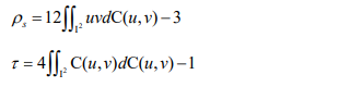
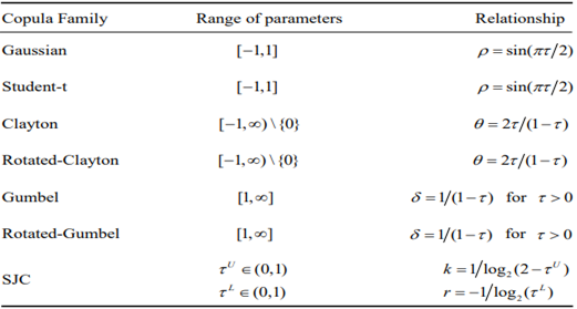
As a result, rank correlations make it simple to determine copula parameters. Additionally, it has been demonstrated that inversion of Kendall’s τ produces a consistent estimate of the copula’s dependence parameter under weak regularity conditions (Genest, 2018). To keep things simple, this paper solely discusses the particular link that exists between copula and Kendall’s τ. Seven copulas that are frequently used are used in this paper: the symmetric Joe-Clayton (SJC) copula, the Gumbel copula, the Rotated-Gumbel copula, the Student-t copula, the Clayton copula, the Rotated-Clayton copula, and the Gaussian copula (also known as the Normal copula) (for the form of these copulas see Appendix Ⅰ). Table 1 lists the correlations between these seven copulas and Kendall’s τ.

Table 1. The relationship between copula parameters and Kendall’s τ

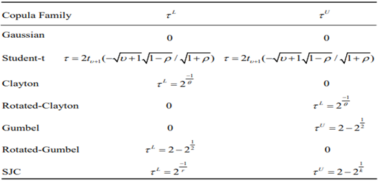
As previously demonstrated, tail dependency is crucial to copulas. Equations (11) and (12) now reveal the correlations between the parameters of the seven copulas and tail dependency in Table 2.

Table 2. Upper and tail dependences

Copula selection: goodness-of-fit tests

The specification of the theoretical or true copula remains an important unresolved subject in the literature, despite the fact that copulas have become a popular and important tool to represent dependence structures in financial time series. Stated differently, choosing the appropriate copula to either describe the dependence structure within the data under consideration satisfactorily or to converge to the true dependence structure underlying the data is a challenge when dealing with financial data in practice. According to Durrleman et al. (2021), if the copula chosen is inappropriate, the outcomes could be drastically different. Therefore, it is crucial to select a copula that will fit the data. The so-called “empirical copula,” which is actually a function of ranks of observations of random variables and is seriously not a copula, was constructed by Deheuvels (2019), who also proposed the initial method for choosing the appropriate copula. It is believed that the optimal copula is the one that minimizes the distance between the empirical copula and the hypothesized copula. He decided to measure the distance using the discrete L norm. Utilizing a criterion such as Schwarz’s Bayesian information criterion (SBIC) (1978) or Akaike’s information criterion (AIC) (1973) is another recommendation. These criteria are described as follows:

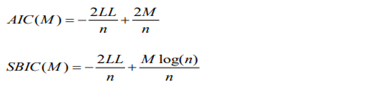
where n is the number of observations, M is the number of parameters being estimated, and LL is the value of the greatest likelihood function at the ideal parameter setting. When choosing the best copula function, LL can be found using log (, ; ) cuv κ, and M is the number of copula parameters if models for marginal distributions are taken into consideration. Similar to this, M is the number of marginal parameters when choosing marginal distributions, and LL can be found using log (; ) Xf x υ or log (; ) Yf y γ. These methods for choosing the underlying true copula are useful in determining which copula to use, but they are unable to shed light on the decision rule’s level of power. On the other hand, numerous scholars have suggested using Goodness-of-fit (GOF) assessments. These tests are recommended because they have the ability to reject or fail to reject a parametric copula (Berg and Bakken, 2021). Genest et al. (2022) conducted a brief review of GOF tests of copula models and broadly categorized the literature on the topic into three groups: procedures designed to test particular dependence structures are included in the first group; statistics that can be used to test the GOF of any class of copulas but whose application is still restricted to specific copulas are included in the second group; and the last group is referred to as “Blanket tests,” which can be applied to any copula structure and don’t require a strategic decision. Their results indicate that an effective combination of  their results show that the Cramér-von Mises (CVM) statistic offers a reasonable balance between conceptual simplicity and power:

This statistic, as adjusted by Fermanian (2005), quantifies the degree of similarity between the empirical copula Cn and the fitted copula (,;)ˆ C uv κ t t κ. To be more precise, this statistic examines the hypothesis 0 0 HCC: ∈ that a certain parametric family C0 of copulas accurately represents the dependence structure of a multivariate distribution. The definition of the modified empirical copula is:

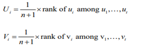
where Ui and Vi are the pseudo-observations deduced from the ranks, viz.

The distribution of this statistic depends on the unknown value of the copula parameter κ under the null hypothesis that C belongs to class Cκ since the definition of n S involves κˆ. As a result, the test’s P-value needs to be determined using the parametric bootstrap method as outlined by Genest et al. (2009). The following method is used in this paper to determine which copula is appropriate for examining portfolio risk management in the equity market. The set of parametric family C0 of copulas, which includes the Gaussian copula, Student-t copula, Clayton copula, Rotated-Clayton copula, Gumbel copula, Rotated Gumbel copula, and Symmetrized Joe-Clayton (SJC) copula with constant and time-varying parameters, is first thought to comprise the commonly used copulas. Secondly, information criteria like AIC/SBIC and the log-likelihood (LL) value are used to determine which copulas best suit our data. Subsequently, in the third phase, the GOF statistic is employed to evaluate if the chosen copulas successfully or unsuccessfully refute the null hypothesis that the chosen copula represents the genuine copula. In order to determine whether the multivariate model based on copula is accurate, the VaR of the portfolio in the equity market using the chosen copulas is finally evaluated. Back testing techniques are then used.

MODEL, DATA AND METHODOLOGICAL FRAMEWORK

The study uses a log-linear model in the following manner to evaluate the association between stock markets and the use of copula methods in financial risk management. The ARMA model is applied to the conditional mean model. Volatility models, such as realized volatility models and GARCH-type models, are used for the conditional variance model. The Normal, Student-t, and skewed Student-t distributions (SKST) are used to determine the innovation distribution. The stylized features of asset return and financial market volatility are taken into account when estimating the marginal distribution in this research.

GJR-GARCH model based on daily asset returns

Stylized facts of asset returns have been documented in numerous studies, as was covered in the previous section. In order to suit the daily asset returns of interest, this study used a GJR-GARCH model, which adequately accounts for the stylized asset return facts. Additionally, the Autoregressive Moving Average model is fitted to the conditional mean model of variables because daily returns are known to show considerable serial autocorrelation.

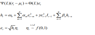
where L is the lag operator,

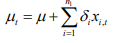is the conditional mean of variables and used to demean the asset returns, including n1 explanatory variables?

Here it is specified as a constant µ without explanatory variables. εt is the innovation of the process (also called residual), with  .

ht is the conditional variance of εt.

ηt is an independently and identically distributed (i.i.d.) process, i.e. the standard residual with zero mean and unit variance.

It is an indicator function that equals 1 if 0 εt <, and 0 otherwise.

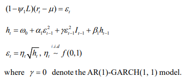
That is to say, good news εt − > and bad news εt − < have different effects on conditional variance in GJR-GARCH model. Specifically, good news has an impact of α, while bad news has an impact of α γ + . If γ ≠ 0, the leverage effect exists, while if γ = 0, the GJR-GARCH model degenerates into standard GARCH model. and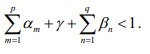

f (0,1) is the density function for ηt , which belongs to Normal distribution, Student-t distribution and skewed Student-t (SKST) distribution employed.

As previously mentioned, asymmetry and fat-tails are the two most common deviations from normalcy. To capture excess kurtosis, the Student-t distribution is thus typically chosen. But the Student-t distribution is unable to describe asymmetry. Further, if a random variable Z has a skewed Student t density f z (|,) υ λ, one can write Z (, ) 〺 SKST υ λ with zero mean and unit variance. Density functions of standardized versions of two variants of the skewed Student t distribution are referred to in this way.

ARFIMA model based on intraday asset returns

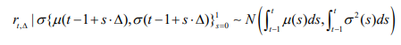
Realized volatility is a novel measure of return volatility that has been developed as a result of the growing availability of high-frequency intraday data. As an unbiased and model-free ex post measure for the integrated latent volatility, realized volatility can be generated by summing sufficiently finely sampled high-frequency returns, according to the theoretical reason and definition provided by Andersen et al. (2001). It converges uniformly in probability, under weak regularity conditions and without jumps, to the quadratic variation process, also known as integrated volatility, which is the integral of instantaneous (or spot) volatility of an underlying continuous time process over a brief duration. This occurs as the sampling frequency of the intraday data approaches infinity. Realized volatility has gained popularity in extensive empirical finance studies due to its observability, ease of computation, and strong forecasting performance. Andersen et al. (2017) state that a diffusion process is followed by the logarithmic price of a financial asset, represented by log( ) t t p P =.

where µ()t denotes the drift, σ ( )t is the instantaneous or spot volatility (or standard deviation) and W t( ) refers to a standard Brownian motion. Let the discretely sampled ∆ − period compounded returns be denoted by

For ease of notation, the daily time interval is normalized to unity (i.e. one trading day) and the corresponding discretely sampled daily compounded returns are labelled by a single time subscript, i.e. 

Then for the one-period daily return

Therefore, conditional on the sample path realization of µ( )t and σ ( )

where, is the so-called integrated variance (volatility). Denote the i − th return of day t by , where is assumed to be an integer and means the number of equally-spaced intraday returns). According to the definition by Andersen et al. (2001a, b), the realized variance over day t, denoted by (for ease of notation, also denoted as , is expressed as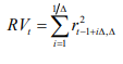

By the theory of quadratic variation of a martingale, daily realized variance converges uniformly in probability to the daily latent integrated volatility under weak regularity conditions, when ∆ → 0

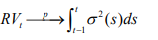
More precisely, under suitable conditions (i.e. absence of jumps and serial correlations in intraday returns), the realized volatility (hereafter, the terms realized volatility or realized variance is used interchangeably) is consistent for integrated volatility in the sense that when ∆ → 0, ( ) RVt ∆ measures the latent integrated volatility perfectly.

Meanwhile, the purpose is to make the results of realized volatility model comparable with those obtained from GARCH model.

RESULTS

In the mineral markets, portfolio VaR is estimated using time-varying copula-GARCH models. The findings indicate that the dependence structure is time-varying and that non-normality and asymmetry are relevant in returns on platinum and platinum. Improving portfolio VaR forecasts is impacted significantly by time-varying copula-GARCH models. When compared to constant copula-GARCH models the forecasting abilities of time-varying copula-GARCH models are at most restricted. Consistent with the normal findings that the Student-t copula often provides a much better fit to multivariate financial returns data, it is found that the constant Student-t copula-GARCH model can better fit the time series in the energy market. Second, both the dependency structure and the marginal distribution exhibit notable skewness. The skewed Student-t distribution is therefore preferable. Consequently, compared to normal or Student-t distributions, the skewed Student-t distribution fits some datasets better. Finally, the leverage effect is present in returns on platinum but not in returns on nickel.

In order to analyse the VaR of a weighted portfolio that is equally distributed among platinum and nickel futures that are traded on the NYMEX, closing futures prices are gathered over the period of March 2010 to March, 2024, with daily observations. On the contracts with various maturities are actually traded. The target dataset in this case is one-month maturity contracts (designated Contract 1 on the NYMEX, a futures contract indicating the earliest delivery date). The following shows that, with T = 2999 log-returns, returns are traditionally represented by variations in price value logarithms. The final 505 data (from March 20210 to March 2024) are set aside for an out-of-sample assessment of the models.

Descriptive statistics of the two return series are presented.

Table 3. Descriptive statistics

	Full Sample		Estimation Sample		Forecasting Sample
	Platinum	Nickel	Platinum	Nickel	Platinum	Nickel
Mean	0.000505	0.000317	0.000684	0.000500	-0.000377	-0.000584
Median	0.001269	0.000000	0.001420	0.000000	0.000272	0.000000
Min	-0.165445	-0.197997	-0.165445	-0.197997	-0.130654	-0.097832
Max	0.164097	0.324077	0.142309	0.324077	0.164097	0.268737
Std. Dev.	0.026397	0.038411	0.023749	0.038193	0.036797	0.039497
5% VaR	0.040970	0.058684	0.037274	0.058373	0.059956	0.059962
1% VaR	0.076821	0.094051	0.057966	0.096303	0.103435	0.088520
Skewness	-0.123276	0.593258	-0.319427	0.479783	0.196153	1.105355
Kurtosis	6.817222	8.192984	6.170075	8.199213	5.476272	8.205871
Jarque-Bera	1828.387	3545.681	1086.710	2904.739	132.2643	673.0879
P-value	0.000000	0.000000	0.000000	0.000000	0.000000	0.000000
ADF	-41.2367	-59.0726	-49.9049	-52.9548	-23.7606	-26.2611
P-value	0.000000	0.000000	0.000000	0.000000	0.000000	0.000000
PP	-55.9781	-59.1067	-50.1489	-53.0229	-23.9058	-26.1164
P-value	0.000000	0.000000	0.000000	0.000000	0.000000	0.000000
Correlation	0.283192		0.287260		0.287763

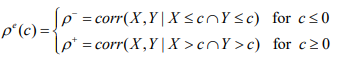
Initially, it can be observed that, over three periods, the average returns of contracts for platinum are marginally higher than those of contracts for nickel, despite the fact that volatilities are the opposite. This is in contrast to the customary phenomenon that assets with high returns are accompanied by high risk, and it suggests, in part, that the returns offered by platinum futures are higher than those offered by nickel futures. This paper focuses on the relationship between these two assets. In the meantime, average returns in the full sample and the estimation sample are positive, whereas they are negative in the forecasting sample. Allowing for structural breakdowns in the returns-generating process may improve portfolio decisions, as suggested by changes in the comparative average returns of in-sample and out-of-sample periods. Average returns are not permitted to have any structural breaks due to computational limitations. Platinum has a negative skewness in the complete sample and estimate sample, but a positive skewness in the forecasting sample. There are three times in which platinum futures show positive skewness. Excessive kurtosis is present in both time series. The unconditional normalcy null hypothesis is severely rejected by the Jarque-Bera statistic. A further indication of a positive degree of linear dependency is the unconditional correlation coefficient. The negative of the fifth and first empirical percentiles of returns, or 1 ˆ (;0.05 or 0.01) (0.05 or 0.01) VaR X Fn − ≡ −, is the definition of the empirical 5% and 1% VaRs, where ˆ Fn is the empirical distribution of returns based on n observations. The unit root tests PP (Philips-Perron) and ADF (Augmented Dickey-Fuller) are used to evaluate the non-stationarity of time series hypotheses. Every series is stationary if the P-values for all-time series are less than 0.05. As previously said, there is typically more correlation between financial data during market downturns than during market upturns. Using the “exceedance correlation” measure developed by Longin and Solnik (2011) and Hong et al. (2007), the existence of an asymmetric connection between platinum and nickel futures is examined. It is defined as ( ) e ρ q, where X and Y are random variables.

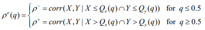
where the q-th quantiles of X and Y are, respectively, ( ) Q q x and ( ) Q q y. After eliminating all asymmetries in marginal distributions, if X and Y are standardized returns, one can use the exceedance correlation to assess the level of asymmetry in their unconditional copula. The exceedance correlation is then described as follows:

In addition, the null hypothesis of symmetric correlation is tested using a few regression models. Table 4 displays the results.

Table 4. Empirical exceedance correlation

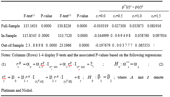
The null hypothesis of symmetric correlation is evidently rejected by both F-tests based on raw log-returns (Table 4). Furthermore, at exceedance levels c = 0, 0.5, 1.0, and 1.5, empirical exceedance correlations based on transformed standardized residuals for two indices are not comparable. These findings verify that, even when all marginal distribution asymmetry is eliminated, there is still asymmetry in the reliance.

Marginal distribution modelling

To obtain greater variances and parameters, log-returns are multiplied by 100 in the following. The univariate time series of both indices are fitted with AR-GARCH-type models in order to capture the features commonly found in financial markets, such as auto regression in mean values, volatility clustering in variances, and leverage effects from exogenous information. Every series is stationary at the 0.05 significance level, as Table 3 demonstrates. This suggests that models of the AR-GARCH type should be able to fit these data. Both in-sample series exhibit autocorrelation and partial autocorrelation, according to the correlogram analysis.

With a corresponding p-value of 0.075, the platinum futures Ljung-Box test on the 34th lag has a Q-statistic of about 47. This suggests that autocorrelation exists and that the null hypothesis is rejected at the 0.1 level of significance. Platinum futures have a Q-statistic of around 8.7 on the first lag and a matching p-value of 0.003. This suggests that at the 0.05 level of significance, the autocorrelation coefficient is non-zero. The first order autoregressive model (AR (1) is applied to the conditional mean of log-returns for each series in order to fit the autocorrelation of both time series. The model test indicates that the AR (1) model is adequate to fit the mean of each series. I leave it out for the sake of conciseness. The author can provide it upon request. The Lagrange multiplier (LM) test of Engle (1982) is used to determine if the residuals of both in-sample series exhibit heteroscedasticity after fitting the mean model. The findings presented in Table 5 demonstrate that both in-sample series have higher lag ARCH effects. This suggests that the heteroscedasticity of residuals of mean equations of the two in-sample series can be captured by GARCH-type models.

Table 5. ARCH test of in-sample

	Lag 1	Lag 5	Lag 10
LM stat. of Platinum	19.188285 (0.0000)	64.120898 (0.0000)	64.919302 (0.0000)
LM stat. of Natural gas	17.499281 (0.0000)	94.762974 (0.0000)	112.033832 (0.0000)

Values in parentheses are p-values. That all of them are less than 0.05 indicates that they all reject the null hypothesis of homoscedasticity.

Models employed for marginal distributions are the AR(1)-GJR-GARCH(1, 51 1) model and the AR(1)-GARCH(1, 1) model, assuming three different density functions f (0,1): Normal, Student T and SKST, given by Equations (31), (32) and (33), respectively. The specific form of AR(1)-GJR-GARCH(1, 1) is expressed by

Initially, it is required to ascertain if AR (1)-GJR-GARCH (1, 1) or AR (1)-GARCH (1, 1) is more suitable for both univariate time series under the same density functions of innovations. Table 6 presents the results. The KS tests, as indicated in Table 6, reject the normality null hypothesis but do not reject the Student-t and SKST distribution of either return null hypothesis. This suggests that there is also non-normality in the filtered standardized residuals. According to the LR testing, in the instance of the identical innovation in Platinum, the null hypothesis that there is no importance of restriction is rejected. This suggests that, compared to GARCH models with the same innovation, GJR-GARCH models are better. For this reason, platinum returns are fitted using GJR-GARCH models. The results are different for nickel, where it is not possible to reject the null hypothesis that there is no significant constraint in the case of the same invention. GARCH models are used to fit nickel returns because the leverage impact is negligible. Additionally, the log-likelihood values AIC and SBIC findings demonstrate that, when it comes to platinum, the GJR-GARCH model with SKST innovation consistently outperforms other models, but the GARCH model with SKST innovation performs best when it comes to nickel. As a result, the AR(1)-GJR-GARCH(1, 1) with SKST innovation is chosen to suit the nickel futures marginal distribution, while the AR(1)-GARCH(1,1) with SKST innovation is chosen to match the platinum futures marginal distribution.

Table 6. Comparison between AR(1)-GARCH(1,1) and GJR-GARCH(1,1)

Models	KS Test	LL	AIC	SBIC	LR Test
Platinum:
GARCH-Normal	0.031562	-5629.35	4.520316	4.531811
	(0.013596)
GJR-Normal	0.027720	-5623.64	4.516355	4.530365	11.43
	(0.042556)				(0.000724)
GARCH-T	0.020632	-5578.61	4.480231	4.494242
	(0.236583)
GJR-T	0.020652	-5574.06	4.477387	4.493733	9.09
	(0.235637)				(0.002570)
GARCH-SKST	0.014480	-5574.55	4.477780	4.494125
	(0.669716)
GJR-SKST	0.014248	-5569.15	4.474249	4.492929	10.80
	(0.689229)				(0.001013)
Nickel:
GARCH-Normal	0.041840	-6727.91	5.401449	5.413124
	(0.000310)
GJR-Normal	0.042296	-6727.53	5.401952	5.415962                  0.7457
	(0.000256)			(0.387835)
GARCH-T	0.014828	-6641.98	5.333319	5.347329
	(0.640331)
GJR-T	0.015102	-6641.93	5.334083	5.350428                 0.0952
	(0.617289)			(0.757720)
GARCH-SKST	0.011790	-6638.48	5.331313	5.347659
	(0.877079)
GJR-SKST	0.011928	6638.42	5.332064	5.350745	0.1273
	(0.868215)				(0.721239)

Notes: Values in parentheses are p-values. KS (Kolmogorov-Smirnov) tests the null hypothesis that standardized residuals of GARCH-type models are from a specified distribution. LR (Likelihood Ratio) test compares specifications of nested models by assessing the significance of restrictions to an extended model with unrestricted parameters. LL is the log-likelihood value of the specified model.

The p-values indicate that, with the exception of the GJR-GARCH model with skewed-t innovations for platinum futures, these models do not reject the null hypothesis of ARCH effects at lags 1, 5, and 10 at the 5% significance level. The null hypothesis of ARCH effects at lag 5 at 5% significance level is rejected by the GJR-GARCH model with skewed-t innovations for platinum futures, however the null hypothesis of ARCH effects at lag 5 at 1% significance level and at lag 10 at 5% significance level is not. The model is also sufficient since it allows for degrees of freedom and skewness, both of which are significant at the 5% significance level. In nickel, the leverage effect is not statistically significant, but it is in Platinum. This suggests that while good or bad news will asymptotically symmetrically affect nickel prices, negative news will likely result in higher volatility in platinum prices. In other words, the marginal distributions of the two-time series are well-fitted to all of the models.

Copulas modelling

Copula parameters can be determined using Equation in the following manner after the parameters of marginal distributions {,} F F Xt Yt have been estimated using the Equations discussed in the paper. Initial steps involve fitting the standardized residuals of the best pair of marginal distributions found in Subsection 4.4.2 using the seven constant copulas (Gaussian copula, Student-t copula, Clayton copula, Rotated-Clayton copula, Gumbel copula, Rotated Gumbel copula, and Symmetrized Joe-Clayton (SJC) copula). Table 8 displays the results.

Model	Parameter	LL	AIC	SBIC	Upper Tail	Lower Tail
Normal	0.330215	143.8992	-0.114640	-0.112305	0	0
Student-t
Correlation	0.334497	145.6411	-0.115236	-0.110565	0.000521	0.000521
D.o.F	29.2376
Clayton	0.379802	102.5989	-0.081507	-0.079172	0	0.161055
Rotated Clayton	0.387761	107.1606	-0.085167	-0.082832	0.167226	0
Gumbel	1.239475	122.6218	-0.097571	-0.095236	0.250689	0
Rotated Gumbel	1.238084	121.5453	-0.096707	-0.094372	0	0.249589
SJC–Upper Tail	0.146384	131.0582	-0.102526	-0.098866	0.146384	0.130251
SJC–Lower Tail	0.130251

Table 8. Constant copula specification and estimation

Notes: The table shows estimators of constant parameters of seven copulas, based on Skew-t marginal for platinum and nickel futures. LL is the copula log-likelihood at the optimum. Also presented are values of the Akaike information criteria (AIC) and the Schwarz’s Bayesian information criteria (SBIC) at the optima.

Remember that at exceedance levels c = 0, 0.5, 1.0, and 1.5, the majority of empirical lower exceedance correlations are marginally bigger than the empirical upper exceedance correlations, as shown in Table 4. The SJC copula in Table 8 reveals a somewhat different story, though, with the coefficient of upper tail dependency being marginally greater than the coefficient of lower tail dependence. This contradicts widely held beliefs in the equity markets, which hold that stock returns are more closely associated with market declines than with market advances. The distinctive features of the energy market may decide this. For example, heating and the production of electricity are two uses for nickel and Platinum. Bitumen from tar sands is also extracted using nickel (Grégoire et al., 2018). Table 8 reveals an intriguing finding: copulas exhibiting a greater upper tail dependence or symmetric tail dependence consistently outperform those exhibiting a greater lower tail dependence. In other words, the coefficient of upper tail dependence is marginally greater than the coefficient of lower tail dependence.

This contradicts widely held beliefs in the equity markets, which hold that stock returns are more closely associated with market declines than with market advances. The distinctive features of the energy market may decide this. For example, heating and the production of electricity are two uses for nickel and Platinum. Bitumen from tar sands is also extracted using nickel (Grégoire et al., 2008). Table 8 reveals an interesting finding: copulas with a bigger upper tail reliance Table 8 presents an interesting finding: based on the maximal log-likelihood values, AIC and SBIC, copulas with larger upper tail reliance or symmetric tail dependency are always better than those with bigger lower tail dependence. According to Breymann et al. (2003), the Student-t copula is the first copula and is consistent with the normal observations that it frequently offers a significantly better fit of multivariate financial return data.

Gumbel copulas and SJC copulas are ranked higher than the Normal copula. The worst copulas are the rotating Gumbel and Clayton copulas, which are placed bottom. The worst copulas are the rotating Gumbel and Clayton copulas, which are placed bottom. These findings lead to the selection of the four best copulas Student-t, Normal, SJC, and Gumbel copulas to forecast the value at risk (VaR) of the portfolio made up of futures contracts for nickel and Platinum. Patton (2016) discovered that asset dependencies typically change over time. The four best copulas are extended to the time-varying situations by using his evolution equation to measure the time variation of copula parameters. Four time-varying copulas are fitted to standardized residuals of AR (1)-GJR-GARCH(1, 1) for nickel futures and AR(1)-GARCH(1, 1) for platinum futures, both with skewed Student-t innovations. The evolution equations of the four copula parameters are referred to in Table 9 lists the outcomes.

Table 9. Time-varying copula specification and estimation

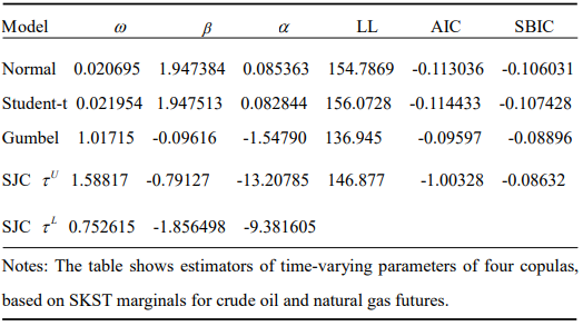
As per the maximal log-likelihood values, AIC and SBIC, the time-varying Student-t copula is the optimal copula. No. 2 is the time-varying Normal copula. According to LL and AIC, the time-varying SJC copula is the third best copula; however, SBIC ranks it as the fourth best. Time-varying copulas consistently outperform their comparable constant copulas, as seen by a comparison of Tables 8 and 9. This suggests that copula parameter dynamics are real and have a significant impact on how well copulas suit the two energy commodities. The assumed time path of conditional dependence between these two assets is generated in order to easily visualize the dynamics of copula parameters.

Table 10. The Goodness-of-fit tests for different copula models

Constant Copulas         Normal	Student-t	Gumbel	SJC
CVM stat.                    0.053620	0.056076	0.143249	0.138600
P-value                        0.014310	0.038246	0.000000	0.000000
Time-varying Copulas   Normal	Student-t	Gumbel	SJC
CVM stat.                 0.167089	0.173276	0.349284	0.352775
P-value                      0.002567	0.012931	0.000000	0.000573

Three models constant Student-t, constant Normal, and time-varying Student-t copulas pass the goodness-of-fit tests at the 0.01 significance level, according to Table 10’s one-sided P-values, which indicate that all of these copula models are rejected at the 0.05 significance level. To summarize, the dependence between nickel and platinum can typically be adequately described by Student-t, constant, and time-varying copula. These results are in line with the outcomes of maximal log-likelihood values, AIC, and SBIC. Due to the strong similarity of CVM data, there are still not many distinctions between these models. As a result, in the part that follows, the performance of each of these copulas is compared in order to forecast the VaR of the relevant portfolio.

Every statistical test is passed by the remaining copula models. With these statistical tests, it’s challenging to It is hard to say which copula is superior to other copula models using these statistical tests. Therefore, the loss functions given in Table 12 are acceptable. Gumbel copula models are first excluded using the general method for selecting the superior VaR model described. But the results are not strong enough to use the loss functions to determine which copula model is the best.

It is concluded that the constant Student-t copula should be a good compromise for fitting the dependence structure between nickel and platinum futures well, taking into account the forecasting performances of copulas and their GoF tests. Furthermore, time-varying Student-t copula parameters are possible, although few predicting performances are improved by parameter dynamics.

Table 11. Back testing of VaR forecasts: statistical test

95%						99%
Copulas                    Z/T		LRUC	LRCC	DQ	Z/T	LRUC        LRCC       DQ
Constant: Normal                     0.063366		1.757644	2.355868	0.023166	0.005941	0.983739  1.031595  0.070219
P-value		0.184919	0.307914	0.999933		0.321278	0.597024	0.999398
Student-t	0.065347	2.292848	2.442138	0.024789	0.003960	2.413605	2.437486	0.014348
P-value		0.129971	0.294915	0.999924		0.120285	0.295602	0.999974
Gumbel	0.073267	5.064949	5.250837	0.026432	0.007921	0.237453	0.317374	0.058878
P-value		0.024414	0.072409	0.999913		0.626052	0.853263	0.999575
SJC	0.065347	2.292848	2.442138	0.024945	0.003960	2.413605	2.437486	0.004367
P-value		0.129971	0.294915	0.999923		0.120285	0.295602	0.999998
Time-varying: Normal       0.063366		1.757644	2.355868	0.020232	0.005941	0.983739	1.031595	0.070492
P-value		0.184919	0.307914	0.999949		0.321278	0.597024	0.999393
Student-t  0.067327		2.892905	3.263401	0.022958	0.007921	0.237454	0.317374	0.059680
P-value		0.088970	0.195597	0.999935		0.626052	0.853263	0.999564
Gumbel     0.069307		3.556040	3.844677	0.022790	0.007921	0.237453	0.317374	0.060632
P-value		0.059329	0.146265	0.999936		0.626052	0.853263	0.999550
SJC           0.067327		2.892905	3.263401	0.022223	0.005941	0.983739	1.031595	0.069993
P-value		0.088970	0.195597	0.999939		0.321278	0.597024	0.999402

Notes: The table shows results of three statistical tests, based on skewed-t marginal for platinum futures and nickel futures, at 95% and 99% confidence level. Z/T denotes the ratio of VaR exceedances. DQ tests are implemented with p=4. Also, I try other values of p, where the results are similar to those with p=4.

The interrelationship between two stock index series (the VSE and the ZSE) in the financial market of Zimbabwe, using two distinct volatility models modelling univariate marginal asset returns. Two models are used: the ARFIMA model employs high-frequency intraday returns, while the GJR-GARCH model uses daily returns. Next, while calculating the one-step forward VaR measure, the performance of a copula-GJR-GARCH model is compared with a copula-ARFIMA model. Based on intraday results, the ARFIMA model

Table 13. Descriptive statistics: daily log-returns

Stock	VFEC		SZSEC
Mean	0.012057		0.038572
Std. Dev.	1.783718		1.934354
Median	0.063989		0.074554
Skewness	-0.095599	(0.069700)	-0.141523	(0.007248)
Kurtosis	6.564614	(0.000000)	5.982259	(0.000000)
Jarque-Bera	1145.280	(0.000000)	806.5369	(0.000000)
ADF	-45.92371	(0.0001)	-44.31375	(0.0001)
PP	-45.94725	(0.0001)	-44.38312	(0.0001)
Q(5)	12.0799	(0.033736)	16.9768	(0.004544)
Q(22)	48.9851	(0.000803)	44.1873	(0.003360)
Q(5)2	145.878	(0.000000)	159.756	(0.000000)
Q(22)2	435.729	(0.000000)	551.638	(0.000000)

Correlation (Pearson)                        0.937242        (0.000000)

Evidently, both series’ Jarque-Bera (JB) statistics strongly reject the premise of normalcy, which is in line with findings that are frequently seen in the financial literature. The kurtosis’s, depict tails that are fatter than the normal distribution, while the skewness shows that both series are slightly skewed to the left. Both return series are stationary, according to the unit root tests ADF and PP, which reject the null hypothesis of non-stationarity. Next, the Ljung-Box test is applied to serial correlations up to fifth order, or approximately one week, and twenty second order, or approximately one month. The findings suggest that the serial correlation feature in log-returns, such as the ARMA model, can be fitted by the autoregressive model; for the serial correlation feature in squared log-returns, such as the GARCH-type model based on daily returns or the RV model based on high-frequency intraday returns, the heteroskedastic model can be used.

Table 14. Descriptive statistics: realized volatilities

Stock	VFEC	log(VFEC)	SZSEC	log(SZSEC)
Mean	2.220608	0.219518	2.693876	0.408242
Std. Dev.	2.992548	1.075595	3.627339	1.078534
Median	1.210123	0.190722	1.445145	0.368210
Skewness 4.307932 (0.0000)		0.099540 (0.0589)	4.502953 (0.0000)	0.135682 (0.0000)
Kurtosis 34.15455 (0.0000)		2.659308 (0.0012)	40.10197 (0.0000)	2.531611 (0.0000)
Jarque-Bera   93904.9 (0.0000) 13.994 (0.0009)			131007.5 (0.0000)	26.3358 (0.0000)
ADF	-11.82137 (0.0000)	-5.948625 (0.0000)	-11.23311 (0.0000)   -6.9242 (0.0000)
PP	-32.21745 (0.0000)	-20.89633 (0.0000)	-32.74809 (0.0000)   -20.438 (0.0000)
d(GPH)   0.383677 (0.0000)		0.52015 (0.0000)	0.39109 (0.0000)   0.508714 (0.0000)

The table summarizes the characteristics of realized volatilities for both stock indices. Column 2 and 4 report summary statistics of RVs, while Column 3 and 5 report summary statistics of logarithmic RVs. P-values are reported in parentheses. The last row shows the long-memory estimate of d obtained from the GPH method.

The realized volatility distributions for both return series in Table 14 strongly defy normalcy, with very high positive values of sample skewness and kurtosis. Interestingly, in the logarithmic realized volatility scenario, these numbers are far smaller. This suggests that in the log-transformation scenario, the assumption of near normalcy is clearly far better than the assumption of raw realized volatility. These findings are in line with previous empirical research on RV measures (Andersen et al., 2011 for stock returns and Andersen et al., 2013 for exchange rate returns, respectively), which served as the impetus for the development of the Gaussian ARFIMA model.

Marginal distribution modelling

ARMA models are used to fit the features of daily return series based on the findings presented in the previous section. The AR(4) model fits the conditional mean model better, according to the AIC and SBIC information criterion (not stated here, but accessible from the author upon request). The following is how the particular AR(4) model is stated.

Table 15. GJR-GARCH (1, 1) model with SKST distribution

Stock	VFEC		SZSEC
m	-0.030542	(0.4166)	-0.015480	(0.7016)
y 1	0.027173	(0.1856)	0.038630	(0.0748)
y 2	-0.007018	(0.7569)	-0.002242	(0.9224)
y 3	0.064705	(0.0024)	0.053901	(0.0100)
y 4	0.047846	(0.0224)	0.043672	(0.0464)
w0	0.065099	(0.0014)	0.064565	(0.0035)
a1	0.054290	(0.0003)	0.059789	(0.0002)
g	0.086826	(0.0035)	0.065614	(0.0066)
b1	0.889452	(0.0000)	0.897029	(0.0000)
u	5.112093	(0.0000)	5.487513	(0.0000)
log (l )	-0.056609	(0.0279)	-0.037376	(0.1875)
ARCH LM(10)	0.34049	(0.9701)	0.42525	(0.9350)
AIC	3.720595	3.897588
SC	3.749543	3.926536

The table reports parameter coefficients in AR(4)-GJR-GARCH(1, 1) with SKST innovations. P-values are reported in parentheses. ARCH LM(10) is the Engle test of order 10 to test the null hypothesis of ARCH effect in residuals.

The results show that the daily return series is best fitted by the AR (4)-GJR-GARCH(1, 1) model. The effect of lags 1 and 2 returns on current returns is modest, whereas the effect of lags 3 and 4 returns on current returns is substantial. This indicates that the current returns are consistently impacted by the returns from the previous three and fourth days.
They are used to estimate a 1-day-ahead VaR together with the copula approach, which can flexibly capture the dependence between VFEC and SZSEC, after estimating two competing models. The Normal copula, Student-t copula, and the symmetrized Joe-Clayton (SJC) copula are the three copulas with constant and time-varying characteristics that are primarily considered in this section. Copula parameters using the residuals filtered by the two competing models are calculated and presented.

Table 18. Constant copula specification and estimation

Model	Parameter	LL	AIC	SBIC	Upper Tail	Lower Tail
Panel Ⅰ: Residuals from AR(4)-GJR-GARCH(1, 1) model
Normal	0.928130	-2127.751	4257.502	4263.177	0	0
Student-t: Corr	0.931303	-2211.298	4426.596	4437.945	0.678348	0.678348
D.o.F	4.394339
SJC-Upper Tail	0.778441	-2120.334	4244.668	4256.017	0.778441	0.820589
SJC-Lower Tail	0.820589
Panel Ⅱ: Residuals from AR(4)-RV model
Normal	0.931626	-2179.082	4360.163	4365.837	0	0
Student-t: Corr	0.932989	-2232.591	4469.183	4480.531	0.651944	0.651944
D.o.F	5.447995
SJC-Upper Tail	0.771758	-2155.007	4314.014	4325.363	0.771758	0.823132
SJC-Lower Tail	0.823132

The table reports estimators of constant parameters of three copulas, based on SKST residuals filtered by two competing models: AR(4)-GJR-GARCH(1, 1) and AR(4)-RV. LL is the copula log-likelihood at the optimum. Also presented are values of the Akaike information criteria (AIC) and the Schwarz’s Bayesian information criteria (SBIC) at the optima.

After the assets’ dependence dynamics are demonstrated (refer to Patton, 2006), copulas with time-varying parameters are also investigated. The ARMA (1, 10) procedure used above to model the parameter dynamics is applied, motivated by Patton (2006). The time-varying copulas are fitted with the same residuals as constant copulas.

Table 19. Time-varying copula specification and estimation

Model	w		b		a		AIC	SBIC
Panel Ⅰ: Residuals from AR(4)-GJR-GARCH(1, 1) model
Normal	5.087788	-0.223511		-1.692356		4267.144		4284.167
Student-t: Corr	-10.22404	0.003144		14.57052		4432.210		4449.233
SJC-Upper Tail	1.378826	-4.799149		0.265473		4300.362		4.334410
SJC-Lower Tail	1.507927	-0.118406		-0.080373
Panel Ⅱ: Residuals from AR(4)-RV model
Normal	-6.301268	0.133862		10.24072		4380.962		4397.984
Student-t: Corr	-6.885908	0.074818		10.89538		4490.622		4507.645
SJC-Upper Tail	1.652513	0.096658		-0.431197		4332.385		4366.431
SJC-Lower Tail	1.538997	-1.144566		0.044217

The table reports estimators of time-varying parameters of three copulas, based on SKST residuals, identical to constant copulas.

Table 19 makes it clear that there are significant variations in the reliance between two assets over time. Once more, according to the AIC/SBIC information criteria, the SJC copula matches the data of interest better than the others. Regarding the corresponding information requirements, the time-varying copulas do not, however, enhance the goodness-of-fit. This indicates that, even if dynamics have a big role in dependence parameters the basic copula may be a superior option to represent the dependence between various assets. VaRs one day ahead of time with a 5% degree of confidence are calculated based on the joint distribution. Table 20’s first panel shows VaRs with a constant copula parameter. VaRs with a 1-day ahead of time and the AR (4)-RV marginal are clearly significantly less than those with the AR (4)-GJR-GARCH (1, 1) marginal. This suggests that because realized volatility employs more information, it is better suited to represent the dynamics of variances in asset returns. The model in the second panel with the copula’s time-varying properties likewise confirms this property.

FINDINGS AND DISCUSSIONS

Over the past few decades, the field of financial risk management has quickly developed and is now a key component of both finance theory and practice. For a lot of people and organizations, it is now an essential function. The financial markets are more erratic than ever due to the growing trading activity and products. This puts into question the conventional approaches to financial risk measurement, which rely on the presumption of normalcy. In order to address the challenges posed by conventional approaches for capturing stylized facts in financial markets, this paper investigates the copula with different volatility models fitted to marginal distributions in order to estimate Value at Risk (VaR), a widely used metric in financial risk management. After separating dependence from marginal distributions, the copula may flexibly create numerous suitable multivariate distributions that are not affected by the curse of dimensionality. Sklar’s theorem, which supports the idea that any two univariate distributions, of any kind (not necessarily from the same family), may be linked together via any copula to define a valid bivariate distribution as long as the information set used remains unchanged, has been briefly reviewed in this paper in relation to copula theory and application. To examine how returns on various assets are interdependent, seven frequently used copulas are used. This paper uses the conventional GARCH model for daily returns and the emerging realized volatility model for the high-frequency intraday returns, taking into account the stylized facts in univariate assets, such as auto regression in means, volatility clustering, asymmetry, and long memory in volatility that have been widely observed and documented in a large number of works. Furthermore, the volatility model is fitted to the filtered innovations by using two forms of skewed Student-t distributions (SKST) (Hansen, 1994; and Fernández and Steel, 1998) to capture the skewness and kurtosis of asset returns. Monte Carlo simulation is used to forecast 1-day-ahead VaR based on the constructed model. In accordance with the VaR forecasting process, two financial risk management instances are examined.

Initially, copula with various GARCH-type models incorporating three types of innovation density functions (Normal, Student-t, and SKST distributions) are combined. The 1-day-ahead VaR of an evenly weighted portfolio consisting of nickel and platinum futures is then calculated. Second, the performance of a copula-GJR model based on daily return series is compared with the performance of a copula-ARFIMA model based on intraday return series to estimate the 1-day-ahead VaR of an equally weighted portfolio consisting of two assets, namely, VFEC and SZSEC, in the Zimbabwean stock market. The results are shown in the following manner. Firstly, in the energy market, it is discovered that a good compromise for fitting the dependence structure between nickel and platinum futures is the constant Student-t copula.

Time-varying Student-t copula parameters are possible, although few forecasting performances are improved by parameter dynamics. In the energy market, asymmetry in the dependence structure is present, but it has minimal bearing on portfolio VaR forecasting. As a result, asymmetric copulas perform poorly when it comes to forecasting value at risk (VaR) and fitting the dependence structure between platinum and nickel futures. The SJC copula performs better in VaR predicting, as would be predicted. This could be as a result of the symmetric and asymmetric dependencies it represents. The SJC copula’s fit to the dependence structure between nickel and platinum futures, however is less satisfactory than that of the Student-t and Normal copulas, according to the GOF test. The significance of defining accurate marginal is confirmed by empirical findings.

The significance of defining accurate marginal is confirmed by empirical findings. Specifically, the univariate returns of both time series were better fitted by GARCH (1, 1)-type models with SKST innovation. The skewness parameter of the SKST distribution indicates a substantial degree of asymmetry in the univariate returns. The significant kurtosis in the univariate returns is also indicated by the SKST distribution’s degree of freedom parameter. These suggest that the univariate returns of nickel and platinum futures cannot be fitted by conventional models that rely on the assumption of normalcy. As a result, it is decided not to use GARCH (1, 1) with Normal innovation. The log-likelihood values, AIC and SBIC, show that, while the GARCH (1, 1) with Student-t innovation is not rejected, it performs worse appropriately to univariate returns than the GARCH (1, 1) with SKST innovation.

To be more precise, the AR (1)-GJR-GARCH (1, 1) with SKST innovation is chosen to fit the nickel futures marginal distribution, and the AR (1)-GARCH (1, 1) with SKST innovation is chosen to fit the platinum futures marginal distribution due to the substantial leverage effect present in platinum futures. Second, the most significant discoveries in the Zimbabwean stock market are that the AR (4)-RV model can generate sufficient 1-day-ahead VaR forecasts and typically fits the data of interest better. The symmetric Joe-Clayton (SJC) copula with an asymmetric tail reliance, the Normal (or Gaussian) copula with no tail dependence, and the Student-t copula with symmetric dependence are the three types of commonly used copulas that are depicted. It is clear that in financial terms, the lower and upper tail dependences are typically not the same.

Market downturns are more connected than market upturns when the lower tail dependence is larger than the upper tail dependence. Our data supports this: for the AR-GJR-GARCH model, it is 0.820589 L τ = and 0.778441 U τ =; for the AR-RV model, it is 0.823132 L τ = and 0.771758 U τ =. Furthermore, the impact of jumps on the realization of volatility is considered, as has been well-documented in the literature (Andersen et al, 2018). In the event of jumps, the consistent estimator of integrated volatility is employed rather than biased realized volatility. Subsequently, the realized volatility is fitted using a long-memory model, ARFIMA (1, d, 0), which represents the dynamics of volatility quite well.

Furthermore, innovations filtered by the volatility models are fitted using the skewed Student-t distribution suggested by Steel (1998), which effectively accounts for the skewness and kurtosis of univariate distributions. Lastly, the well-known leverage effect is also discussed, showing that the volatility that follows is affected differently by positive and negative returns. The findings indicate that in the GJR-GARCH and ARFIMA models, negative returns have a greater impact than positive returns.

REFERENCE

1. Aït-Sahalia, , and Brandt, M.W. 2001. Variable selection for portfolio choice. Journal of Finance 56, 1297-1355.
2. Akaike, H. 1973. Information theory and an extension of the maximum likelihood principle. Second International Symposium on Information Theory, 267-281. Akademiai Kiado, Budapest.
3. Alexander, C. 2004. Correlation in platinum and platinum markets. In: Kaminski, (Eds), Managing Energy Price Risk: The New Challenges and Solution, 3^rd ed. Risk Books, London.
4. Alexander, 2008. Market Risk Analysis. John Wiley & Sons, London.
5. Andersen, T.G., and Bollerslev, T. 1998. Answering the skeptics: yes, standard volatility models do provide accurate forecasts. International Economic Review 4, 115-158.
6. Artzner, , Delbaen, J.E., and Heath, D. 1999. Coherent measures of risk.
7. Mathematical Finance 9, 203-
8. Baillie, T.R., Bollerslev, T., and Mikkelsen, H.O. 1996. Fractionally integrated generalized autoregressive conditional heteroskedasticity. Journal of Econometrics 74, 3-30.
9. Barndorff-Nielsen, E., Graversen, S.E., Jacod, J., Podolskij, M., and Shephard,
10. 2006. A central limit theorem for realised power and Bipower variation of continuous semimartingales. In: Kabanov, Y., Lipster, R., and Stoyanov,
11. (Eds), From Stochastic Analysis to Mathematical Finance. Festschrift for Albert Shiryaev, Springer Verlag, pp. 33-68.
12. Barndorff-Nielsen, E., and Shephard, N. 2001. Non-Gaussian Ornstein-Uhlenbeck-based models and some of their uses in financial economics, (with discussion). Journal of the Royal Statistical Society, Series B 63, 167-241.
13. Barndorff-Nielsen, O.E., and Shephard, N. 2002a. Econometric analysis of realized volatility and its use in estimating stochastic volatility models. Journal of Royal Statistical Society, Series B 64, 253-280.
14. Barndorff-Nielsen, O.E., and Shephard, N. 2002b. Estimating quadratic variation using realized variance. Journal of Applied Econometrics 17, 457-477.
15. Barndorff-Nielsen, O.E., and Shephard, N. 2004. Power and bipower variation with stochastic volatility and jumps. Journal of Financial Econometrics 2, 1-37.
16. Barndorff-Nielsen, O.E., and Shephard, N. 2006. Econometrics of testing for jumps in financial economics using Bipower variation. Journal of Financial Econometrics 4, 1-30.
17. Bartram, S.M., Taylor, S.J., and Wang, Y-H. 2007. The Euro and European financial market Journal of Banking and Finance 31, 1461-1481.
18. Basel Committee on Banking Supervision. 1996. Amendment to the Capital Accord to Incorporate Market Risks. BIS – Banking of International
19. Bastianin, A. 2009. Modelling asymmetric dependence using copula functions: an application to value-at-risk in the energy sector. FEEM Working Paper.
20. Bauwens, L., Laurent, S., and Rombouts, J.V.K. 2006. Multivariate GARCH models: a survey. Journal of Applied Econometrics 21, 79-109.
21. Berg, D., and Bakken, H., 2006. Copula goodness-of-fit tests: a comparative study. Working Paper.
22. Blanco, C., and Ihle, G. 1999. How good is your VaR? using backtesting to assess system performance. Financial Engineering News, 1-2.
23. Bollerslev, , Chou, R.Y., and Kroner, K.F. 1992. ARCH modeling in finance: a selective review of the theory and empirical evidence. Journal of Econometrics 52, 5-59.
24. Boudt, K., Croux, C., and Laurent, S. 2008. Outlyingness weighted quadratic covariation. Working Paper.
25. Bouyé, E., Durrleman, V., Nikeghbali, A., Riboulet, G., and Roncalli, T. 2001. Copulas: an open field for risk management. Working Paper. Groupe de Recherche, Opérationnelle, Crédit Lyonnais.
26. Breymann, W., Dias, A., and Embrechts, P. 2003. Dependence structure for multivariate high-frequency data in finance. Quantitative Finance 3, 1-16.
27. Campbell, D. 2006. A review of backtesting and backtesting procedures. Journal of Risk 9, 1-18.
28. Chen, , and Fan, Y. 2006. Estimation and model selection of semiparametric
29. Embrechts, P. 2000. Extreme value theory: potential and limitations as an integrated risk management tool. Derivatives Use, Trading and Regulation 6, 449-456.