Development of a Probabilistic Cost Model for Well Intervention Cost Estimation

 Development of a Probabilistic Cost Model for Well Intervention Cost Estimation

Morgan Manuchim WOPARA^1*, Joseph AJIENKA¹, Alwell NTEEGAH¹, Erasmus NNANNA²

¹Emerald Energy Institute (EEI), University of Port Harcourt, Rivers State, Nigeria.

²Shell Petroleum Development Company of Nigeria, Port Harcourt, Nigeria.

DOI: https://doi.org/10.51244/IJRSI.2024.1105066

Received: 07 May 2024; Revised: 15 May 2024; Accepted: 20 May 2024; Published: 20 June 2024

ABSTRACT

Accurate cost estimates are crucial for assessing the commercial viability and business case of well intervention projects, considering the limited available resources. This study presents the development of a comprehensive cost estimation model tailored specifically for rigless well intervention projects. We used the probabilistic approach to develop a cost estimation model for well intervention to achieve the research objective. The developed cost model was transformed into a computer program using pseudocodes in the C-Sharp programming language. The costs of well interventions performed on five (5) wells were used to validate the well intervention cost estimation software. We compared the cost estimation results using the Well Intervention Cost Estimation software and an existing deterministic cost estimate. For every cost estimate that the software generates, three probabilistic values are calculated (P90, P50 and P10). The cost-estimating application resulted in a higher cost than the deterministic estimate because it accounted for project uncertainties. As a result of implementing this cost estimation model, oil and gas industry cost analysts can optimize resource allocation, improve project planning, and mitigate financial risks associated with well interventions, thus improving operational efficiency and profitability.

Keywords—Well Intervention, Cost Estimation, C-Sharp Programming, Oil and Gas Industry, Cost Estimation Model Development.

INTRODUCTION

Oil and gas wells seldom operate effectively and produce continuously from the time of production until they are abandoned.  The well will eventually have problems on the surface or at the subsurface. Well intervention solves these well underperformance concerns [1]. As oil and gas fields get older, well intervention activities become more intensive in the oil and gas industry.

[2] defined well intervention “as any operation performed on an oil or gas well at or towards the end of its productive life that modifies the well’s condition or geometry, offers well diagnostics, or regulates the well’s output.” This means that well interventions are performed to restore a shut-in well to production, optimize production from flowing wells, or for data acquisition. Well intervention is a technique for extending the life of wells to meet the increasing global oil and gas demand [3]. Of course, drilling new wells all the time is a capital-intensive project. Hence, there is a need to restore existing wells to production and optimize production from flowing wells. Well, intervention accounts for over five per cent of global oil and gas production annually.

Oil and gas well intervention projects involve various activities aimed at enhancing or restoring the productivity of existing wells. Oil and gas well intervention projects involve various activities aimed at enhancing or restoring the productivity of existing wells. These projects can include well maintenance, workover operations, and interventions to improve or restore production. The costs related to well intervention tasks may fluctuate based on various factors, such as the type of intervention, well intricacy, geographical location, and specific objectives of the project. Cost estimation is critical to the success of well intervention projects because it determines the commercial viability and the business case of selected projects owing to the limited available resources. The accuracy of a cost estimate is important because it helps establish the project budgets and serves as a tool for scheduling, evaluating, and controlling the project’s cost [4]. The accuracy of the estimated cost is directly proportional to the definition of the project scope and its alignment with actual execution [5].

Well intervention cost models are usually developed using a deterministic approach. This approach is generally based on the definition of the project scope, available historical data, and the contractors’ quotation for that project. The challenge with this approach is that it results in a single-point estimate, which does not account for the uncertainties in the project execution [6]. As a result, the accuracy of the estimated cost is limited because cost-impacting factors are not considered in the estimate. [7] also noted that using a deterministic approach to predict costs might lead to substantial underestimation of prospective cost by the misuse of the “contingency factor,” neglecting the variations costs of line items, lack of understanding of the consequences and likelihoods of probable risk occurrences and by adding non-explicit (extra) contingency to base costs and the total contingency.

Well intervention project risks and uncertainties might come from different sources. For example, [8] and [9] noted that cost overruns in oil and gas projects may result from unclear scope of work, poor contract management, changes in site conditions, unrealistic contractor prices, and delays in material delivery. Information concerning uncertainties and their features, such as higher or lower values, ranges of quantities, and prospective costs, cannot be readily considered in the deterministic method even though this information is readily available or may be calculated.

On the other hand, the probabilistic approach uses best-fit distributions of probabilities to account for the risk and uncertainty in the cost estimate. One of the main benefits of probabilistic cost estimating approaches is the ability to provide clarity into the estimate’s precision, as well as the influence of uncertainties and the risk of cost overruns. A probabilistic technique may be used to create cost-estimating models that take project execution risks into account. This method will account for the variables that lead to cost overruns, resulting in a more accurate and realistic estimate of the well intervention project expenses.

Previous research in oil and gas project cost estimation using a probabilistic approach tends to concentrate on drilling costs, facilities, decommissioning, and abandonment costs. For example, [10] developed a cost estimation model for determining drilling project costs, [11] developed a cost estimation model for the accurate determination of production facilities cost, [12] developed a cost estimation model for evaluating plug and abandonment project costs, while [13] developed cost estimation model for decommissioning of oil and gas projects.

It may be determined that cost estimation modelling for well intervention projects has received less scholarly attention. No empirical work on well intervention projects has focused on developing a tool for a probabilistic cost estimation model. Hence, this study seeks to develop a cost estimation model for well intervention project costs using a probabilistic approach and a C-programming tool.

LITERATURE REVIEW

Cost estimation is very important to effectively manage oil and gas project costs and schedules considering limited resources. As a result, several empirical cost estimation models were developed for different projects in the oil and gas industry. For example, [14], [15], [16], [17], [18] and [19] developed cost estimation models for determining drilling and well construction project costs. [20] developed a cost estimation model to accurately determine production facilities’ costs, while [21] developed cost estimation models for decommissioning oil and gas projects.

Though these models were developed to estimate costs in different upstream oil & gas projects, some gaps still exist in most of the studies. For example, some models were developed using a deterministic approach and did not account for the project cost overruns [22]. Some studies considered the impact of uncertainties, but the models were not specified ([16], [17]). The model developed by [23] considered the effects of risks, but it did not incorporate causes of cost overruns, and the probability distribution criteria were not defined. The model [14] developed was not validated with historical data, and the uncertainties of the project were not incorporated. The basis for selecting the probability distributions was wrongly specified in some of the models [18].

The method used in some of the studies aligns with the intended approach of the current research ([10], [24]). The result will yield a probabilistic cost estimate indicating the value for the low case, base case, and high case cost estimate for the project under consideration.

[15] published Probabilistic Drilling-Cost Estimating and described how the company used the method to estimate drilling costs. Conoco well engineers developed a drilling cost forecasting spreadsheet utilizing a model that incorporated risk analysis and Monte Carlo simulation together with regional cost data since risk analysis has grown to be an important factor in the decision-making process in the petroleum sector. The spreadsheet separated the primary feature categories into two groups and offered a query sort for each. The Big-Rock Sort was the name given to the first group. Those characteristics were the primary cost drivers for this collection of features, which accounted for 80% of the overall cost estimate. The probabilistic technique was used to deal with the relatively few characteristics in this group. The uncertainty for these aspects was described in further detail. The second group consisted of little rocks, easily handled using a deterministic strategy by inputting discrete numbers into a spreadsheet.

The separate well models could not, however, be added together to produce this. It was necessary to do a higher degree of Monte Carlo simulation utilizing the input of the distribution of individual wells. To comprehend the unpredictability of the well construction process, the model for the specific well was first constructed. The model has then divided into 7 batch phases: the top hole, a 1214″ pilot hole, a sidetrack 12 14″ main bore, an 8 12″ hole, a good test, an upper completion run, and an operation to run a subsea Christmas tree. The statistical distributions used in the MCS as an input to construct the complete field simulations for duration and cost are derived from the simulation results from each operating phase of the campaign. This study emphasized the learning impact and correlation of comparable activities, but additional research was needed to apply this using a probabilistic approach.

[17] examined the use of probabilistic analysis to assess new technology’s advantages. Most of the time, historical data wasn’t accessible for developing technology. In those situations, analyzing the impact and utility of the technology using a probabilistic approach was arguably the best and most appropriate course of action.

Although the use of the probabilistic technique and Monte Carlo simulations for well-cost prediction has been introduced for a considerable amount of time, this study noted that very little published work has been done on the subject. The survey was done, and its findings showed that the absence of regular training and refresher courses for pertinent people was one of the major barriers to the widespread use of probabilistic approaches.

[24] developed The Risk€ program to introduce and deepen the use of probabilistic well cost estimates. The well construction procedures are broken down into several smaller activities by the model employed in this programme. The sum of the costs and times for each sub-operation makes up the overall cost and time. Using this model makes it possible to evaluate different well designs in terms of cost uncertainties. Unwanted occurrences were included in the well-building process regarding their likelihood of happening and the length of time they would add. The findings were then provided in two different formats, namely, the risk operation plan with undesired occurrences included and the normal operation plan without unpleasant events.

The development of a spreadsheet model for the probabilistic model for calculating drilling time and cost in Statoil was described by Hollund et al., in 2010. The model discussed in this study included estimate and risk management when data weren’t readily available, combined with statistical techniques drawn from a sizable database. A breakdown of the well model’s number of drilling operations was done. The model was then calibrated to historical data using location, geology, technology, and era information. After that, an outlier algorithm was used to verify the data. Drilling and Well Estimator (DWE), a piece of software created due to the project, was integrated into the company’s database. To improve the accuracy of all Statoil drilling and well operations, this program will be utilized for time and cost estimation. As a result, the delivered wells’ proximity to estimates in the planned wells has been improving. The use of learning curves for cost estimates has evolved into a best practice among many operators, according to a 2011 study by

[25] analyzed performance in terms of cost and length suitable for drilling and completion campaigns of multiple wells. Thus, failing to include the learning curve’s impact might result in an overly negative prognosis. Additionally, they suggested a three-step process for using the learning curve in probabilistic cost estimates.

First, the standard probability analysis is done. The learning impact is not considered in this phase. It is implemented in the second phase, either deterministically or probabilistically.

[26] applied a formulation to estimate the parameters of the learning equation and noted that it has little uncertainty, making deterministic learning suitable. Probabilistic learning is more appropriate if significant uncertainty exists in one or more parameters. The final step is to modify the simulation’s outcome. As the wells are being operated, the initial probabilistic estimate obtained in the first phase must be revised.

Scholars have written on the literature of cost estimation and management in different fields. In the oil and gas industry, some of the scholars have written on cost estimation in drilling and well construction, facilities, field development and decommissioning but few scholarly literatures exist on well intervention project cost estimation. The limitation of the existing models is that some were developed with a deterministic approach which does not consider uncertainties resulting in cost overruns in the project. Other models that were developed with a probabilistic approach were either not correctly specified or the bases for the probability distributions in the model was not justified. Hence, the current study seeks to address these gaps by developing a cost estimation model for well intervention projects that will consider the uncertainties that result in cost overruns using a probabilistic approach.

METHODOLOGY

A probabilistic cost estimation model for well intervention is developed to accomplish the research objective. A C-Sharp programming language is used to write pseudo codes that will transform the probabilistic cost estimation model into a computer programme that will be used for estimating well intervention project cost. The cost elements, work breakdown structure and associated uncertainty are identified for the selected well intervention operation. The C-Sharp programming language helped to create a user-friendly interface for cost estimation. The user interface aided in the selection of the sequence of operations and activities for a selected intervention type. A probability distribution is allotted to each of the cost elements associated with each activity. The probability distribution chosen will be fully justified based on the central limit’s theory. After the cost elements are identified and their probability distributions are specified, a Monte-Carlo simulation would be run for a selected number of trials. The result of the simulation generated the estimated cost for the selected intervention type based on the low case, base case, and high case. We validated the model using existing well intervention project cost data. By following these measures, we can ensure that the model is suitable and reliable for estimating oil and gas well intervention costs.

A.      The Cost Estimation Model

The well intervention activities are broken down into several sub-operations for which the time and costs will be described using probability distributions. In other words, specialists in the well intervention process will give the variation in cost and the number of days for each operation. The summation of the costs and times for the individual operations will then represent the overall cost and time for the project.

Equations (1) and (2) provide the mathematical expression of the process assuming no downtime factor is expected in the operations:

D_T is the total number of days for the well intervention.

D₁, D₂, D₃ …, Dy are the number of days for executing operations 1, 2, 3 …, y respectively and y is the number of each operation.

Considering that well intervention projects cannot be executed without downtime, we factor the downtime expected from executing the operation and that of unfavourable weather conditions into the equation.

Therefore, Equation (2) is rewritten as:

D_i is the number of days for executing operations i for i = 1, 2, 3 …, n respectively

di is the downtime resulting from executing each operation i for I = 1, 2, 3 …, n respectively.

d_w is the downtime resulting from unfavourable weather.

The cost model is provided in Equations (4) and (5):

C_f is the total well intervention project cost.

C₁, C₂, C₃ …, C_y are the costs of executing operations 1, 2, 3 …, y respectively and y is the number of each operation.

The cost of each operation is determined by the rate and days.

Therefore, the total project cost for the well intervention is written as:

Ri is the rate associated with executing each operation i for I = 1, 2, 3 …, n respectively.

r_i is the rate associated with the downtime resulting from executing each operation i for I = 1, 2, 3 …, n respectively.

r_w is the rate associated with the downtime resulting from unfavourable weather.

B.      Monte Carlo Simulation Overview 

Monte Carlo simulations are particularly valuable when dealing with systems that involve multiple sources of uncertainty or when the system’s behaviour is too complex to model analytically. The accuracy of Monte Carlo simulations depends on the number of simulations performed; more trials typically lead to more accurate results. However, the computational cost increases with the number of simulations, so there is often a trade-off between accuracy and computational resources. A well intervention may be divided into several input phases. Each step will have an element of uncertainty connected with the intended, effective time required to complete it. A probability distribution is constructed for each of these uncertain inputs, describing the ranges of potential times for a given step and how likely each conceivable time will occur within this range. The definition of this probability distribution is a crucial step in the procedure.  Uniform distribution and triangular distribution are used for the purpose of this research to account for the different uncertain parameters.

A variety of probability distributions are available to fit offset data. The development of well and time cost models using triangular and uniform distributions has grown to be generally accepted. The uniform distribution is the most straightforward because it simply has a minimum value and maximum value to describe it. Triangular distribution broadens uniform distribution by including a most likely value.

In a uniform distribution, all possible values within a specified range have an equal chance of occurring. The probability density function remains steady over the range and zero outside it. The distribution is defined by its minimum and maximum values. This distribution is useful when there is no specific knowledge about the likelihood of different outcomes within the range. A random variable with constant probability over an interval has a uniform distribution, or f(x), with constant probability. It is occasionally referred to as a random distribution, a “rectangle” distribution, or a “boxcar” distribution. The two main parameters that characterize this distribution are a and b, which stand for their lowest and maximum values, respectively.

Three factors describe the triangular distribution: the mode (the most likely value), the maximum, and the minimum. The continuous probability distribution known as the triangle distribution, which has its lowest value at a maximum value at b, and peak value at c, is sometimes described by the terms lower limit, upper limit, and mode. It’s possible to have both symmetry and skewness. It is often used when there are few samples of data available, particularly when there is an obvious relationship between the variables but there is less data.

Instead of selecting the best distribution, time should be spent making sure the input distributions accurately reflect the mean and spread of the offset data under analysis. The mean and deviation from the mean (Standard deviation) are the two components of input distributions that, according to Purvis (2018), are transmitted through a model to the final output.

Central Limit Effect and Correlation 

Understanding how the Central Limit Theorem might impact a model while creating one is crucial. The Central Limit Theorem is arguably the most significant theorem for risk analysis modeling Vose (2008). According to the theory, a normal distribution with a gradually decreasing standard deviation will result from the sum of all probability distributions, regardless of their shape. If ignored, this can produce absurdly limited outcomes.

The Central Limit theorem can be mitigated in three primary ways to prevent overly narrow results.

Limit the number of input variables. Fewer than fifteen input stages should be used, according to various unpublished sources. This could be feasible, but it severely restricts how the additional advantages of utilizing a probabilistic method are realized, making it a less-than-ideal solution (Kim, 2011)

Avoid utilizing input ranges that are too constrained, and don’t underestimate uncertainty. Although it has already been said, it is important to emphasize that input variables should have realistic minimum and maximum values.

Use correlation to Introduce interdependence between the input variables. A model with no connection presupposes that every single occurrence is independent. The addition of correlation will result in a more realistic range of outputs because experience has taught us that this is rarely, if ever, an accurate picture of reality.

C.      C-Sharp for Developing Cost Estimation Application

Various processes are involved in creating a cost-estimating application in C-Sharp, starting with designing the user interface and ending with implementing the logic for cost calculation. A broad overview of how to approach this procedure is provided as follows:

Project Organization: Using your favourite development environment (such as Visual Studio), start a new C# project. Pick the appropriate project template depending on the kind of program you’re creating (such as Windows Forms, WPF, or a console application).

Designing User Interfaces: Select the layout for the user interface. Let’s say you’re making a Windows Forms application for simplicity. Labels, text boxes, buttons, and perhaps a list view or data grid are among the drag-and-drop components that can show results. Make the user interface (UI) capable of accepting user input, such as item names, quantities, and unit pricing.

Handling User Input: Create event handlers for UI control events, such as button clicks. Store the item name, quantity, and unit cost information the user submits in variables or data structures.

Cost Estimation Logic: Create a class or structure to represent an item. This class should have attributes for the item name, quantity, and unit price. Save an instance of this class for each item that the user enters.

Mathematical reasoning: Use logic to determine the overall cost of each item. The amount and unit cost can be multiplied to achieve this. To determine the overall anticipated cost, add up the expenses of all the products.

Results Display: Fill up any list views or data grids you’re using with the details of the objects and their determined costs. At the bottom of the UI, display the entire expected cost.

Handling Errors: To detect incorrect input, including negative numbers or non-numeric cost values, implement error handling. Show the user the proper error messages to help them.

Improvements: Offer formatting and currency selection possibilities. The option to store and load cost projections from files or a database should be included. Add a clear/reset option to let users start with their estimates again.

Evaluation: Extensively test the programme to ensure it appropriately estimates expenses and can adapt to various conditions. Look for edge cases, incorrect input, and different input combinations.

Deployment and documentation: Explain the function of each method, class, and crucial logic in your code documentation. Converting your programme to an executable or distributable package may prepare it for distribution. Distribute the software to consumers or make it available on pertinent platforms (such as the Windows Store or workplace intranet).

User Experience: Optional: Consider including tools like autocomplete for item names, tooltips, and keyboard shortcuts to improve the user experience.

RESULTS

The cost estimating application is a desktop-based application which is installed on a laptop or desktop and runs on Windows. The software is an executable file, making it easier for user installation. The application has access to a local file system for creating new files, saving, and opening existing files. The application is built to run offline, so it does not require an internet connection.

The tool has seven basic tabs for different functionalities, and they include the preliminary information, the cost information, the equipment summary, the operation charges, the cost estimation, simulation results and chart results. The basic functionalities of the well intervention cost estimating tool are described below:

Preliminary information: This is the tab where the user enters basic information about the projects such as field name, location, number of days for the operation, and the cost estimator’s details.

Cost Information: This tab enables the user to enter the cost of personnel that would be involved in the well intervention campaign. The number of personnel the rate per day and the number of days are entered by the user to calculate the cost of the team members.

Equipment Summary: This tab enables the user to enter the cost of the equipment that would be used for the well intervention campaign. The equipment type, rate per day and the number of days is entered by the user to calculate the cost of each equipment.

Operational Charges: On this tab, the user specifies the type of well intervention services that would be carried out and enters the cost of each service.

Cost Estimation: This is the tab where all the analysis is carried out. The results of the uncertain parameters obtained from the statistical analysis of the research questionnaire on causes of cost overruns for well intervention projects are displayed on this tab. Each of the uncertain variables is assigned a Monte-Carlo distribution which the user must choose for the variables. The set-up comprises of the uncertain parameters which are simulated based on a uniform or triangular distribution. Uniform distribution requires two inputs, minimum value, and maximum value of the uncertain parameters. The triangular distribution requires three inputs, minimum, maximum and mode value of the uncertain parameters. The estimated number of days for the project is also entered on this tab for the application to automatically calculate the cost per day. The user also must enter the value for the number of iterations and the interval for the iteration. The number of iterations should be at least 10,000 for better simulation results. The interval should be at least 50 and it’s selected from the number of iterations entered. Once all these parameters are entered, the user can then click the Run button for the simulation to run.

Simulation Results: This tab is where the result of the simulation is displayed in a tabulated format. The result of the simulation shows the probability of each of the uncertain parameters for the different variables selected as uncertainties. Since at least 50 iterations are selected, the result will display up to 50 different probabilistic values for all the parameters chosen.

Chart Results: This tab displays the simulation’s results as a Probability Density Function (PDF) on the left and a Cumulative Density Function (CDF) on the right. The PDF shows the histogram of each of the uncertain parameters while the CDF shows the plot of probability versus cost of the well intervention project. The user can hover over the CDF plot curve to see the result at different probabilistic levels. However, the P10, P50, and P90 values are displayed in the chart automatically by the software. It is recommended to use the P50 cost estimate for budgeting purposes.

Help: Clicking the note tab will enable the user to access the help/guides required to navigate the software and receive relevant information. Click the Cancel button when presented with the license notice.

Option Menu:

The option menu is located at the top left corner of the application, and it comprises of

• New: for creating new analysis
• Open: for importing existing analysis in .wce format
• Save: for saving an analysis for later use.

Details of the various menus of the well intervention cost estimating software are shown in Fig. 1

A.     Software Application Workflow

To use the well intervention cost estimating software, the user must create new project by clicking the file from the menu bar and choosing “New”. After that, enter the required input data for the preliminary information, cost information, equipment summary and service operation charges. Once all this information is entered, you need to setup the Monte-Carlo simulation run. This is where you select either uniform or triangular distribution depending on the uncertain parameter. Users also need to input the number of days estimated for the operation and the software will calculate some of the inputs automatically. The number of iterations is also selected including the intervals of the result to be displayed. Once all the inputs are set up accurately, you click on run and view the results in the chart menu. Parameters can be modified to re-run the simulations. The cumulative density curve will display the P10, P50 and P90 values of the cost estimate. It is recommended to use the P50 estimate as the basis for the total cost of the well intervention project. A summary of the workflow is shown in Fig. 2.

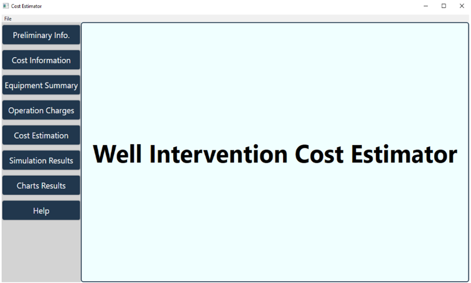
Fig 1: User interface of the well intervention cost estimation software.

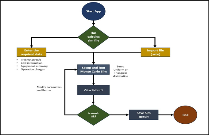
Fig 2: Well intervention cost estimating software workflow.

B.     Model Application

The cost of well intervention performed in five (5) wells was used for the validation of the well intervention cost estimation software. Perforation addition and nitrogen lifting was carried out in well 1 and well 2.  Squeezing, re-perforation and nitrogen lifting was executed in well 3 while Water Shutoff, Perforation Addition and Nitrogen Lifting was performed in well 4 and well 5. Table 1 shows the results of the cost estimation analysis on five (5) well intervention projects using the Well Intervention Cost Estimation software and the result from an existing deterministic cost estimate. For each estimate generated by the software, three probabilistic values were calculated (P90, P50 and P10). Table 1 shows the results of the cost estimation analysis.

Table 1: Results Cost Estimation using Well Intervention Cost Estimation Software and the Result from an Existing Deterministic Cost Estimate.

	Deterministic Estimate		Probabilistic Estimate from the Software
	Total Cost (USD)	Contingency (10%)	P90	P50	P10
Well 1	1,035,036	1,138,539	1570000	1490000	1500000
Well 2	1,402,956	1,543,252	1790000	1820000	1830000
Well 3	1,663,643	1,830,008	2010000	2040000	2030000
Well 4	817,882	899,671	1640000	1600000	1670000
Well 5	1,201,496	1,321,646	1300000	1350000	1200000

Fig. 3 shows the result of the comparison of the existing deterministic cost estimate versus the probabilistic estimate (P50) calculated from the Well Intervention (WI) software. The P50 estimate is relatively higher than both the total cost and the 10% contingency cost because the estimate from the software considered the various factors that impacts on well intervention projects. This means that the factors resulting to cost overruns were included in the calculated costs from the software.

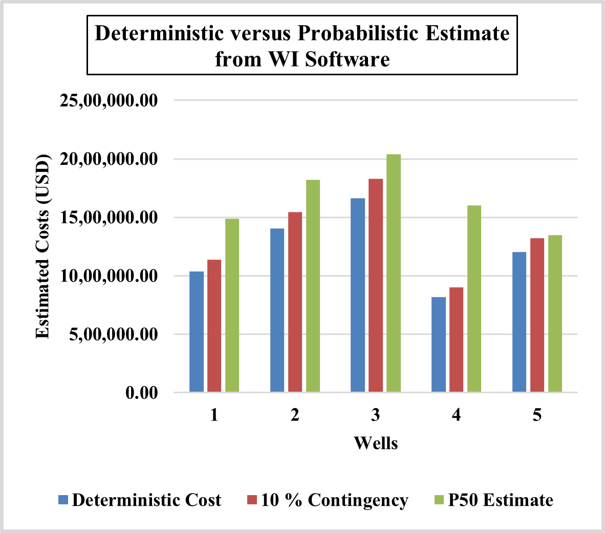
Fig 3: Comparison of the existing deterministic cost estimate versus the probabilistic estimate (P50) calculated from the Well Intervention (WI) software.

CONCLUSIONS

Accurate cost estimates are crucial for assessing the commercial viability and business case of well intervention projects, considering limited available resources. The accuracy of cost estimates depends on well-defined project scopes and alignment with execution expectations, serving as a tool for project budgets, scheduling, evaluation, and cost control.

The cost estimating application is a desktop-based application which is installed on a laptop or desktop and runs on Windows. The software is an executable file, making it easier for user installation. The tool has seven basic tabs for different functionalities, and they include the preliminary information, the cost information, the equipment summary, the operation charges, the cost estimation, simulation results and chart results, and the help menu.

The cost estimating application resulted in a higher cost than the deterministic estimate because it accounted for the project uncertainties.

REFERENCES

1. Mahmood, S. F. (2020). Brownfield projects cost & schedule optimization. Paper SPE-203110-MS presented at the Abu Dhabi International Petroleum Exhibition & Conference to be Held in Abu Dhabi, UAE, 9 – 12 November 2020.
2. Munkerud, P. K., &Inderberg, O. (2007). Riserless light well intervention (RLWI). Paper presented at the Offshore Technology Conference Held in Houston, Texas, U.S.A., 30 April – 3 May 2007.
3. Setiawan, T., Ghazali, R. B., Granados, L. P., Sepulveda, W., Chandrakalatharan, J., Zubbir, A. U., Hanafi, M. M. M., Vaca, J. C., & Yildiz, R. (2016). Samarang well intervention performance evaluation for production enhancement portfolio. Paper SPE 180689_MS presented at the IADC/SPE Asia Pacific Drilling Technology Conference, Singapore, 22-24 August 2016.
4. Ammar, A., Abdullah, L., Helmi, S. A., Zuhra, A., Kadir, A., & Hisjam, M. (2018). Cost estimation model of structural steel for super structure of wellhead platform in oil and gas industry. Paper presented at the Proceedings of the International Conference on Industrial Engineering and Operations Management, Bandung, Indonesia, March 6-8, 2018.
5. Omar, M. S. (2013). Cost estimation for building construction projects in gaza strip using artificial neural network (ANN) (Unpublished Master’s Thesis).
6. Geberemariam, T. K. (2018, November 12). Deterministic and Probabilistic Engineering Cost Estimating Approaches for Complex Urban Drainage Infrastructure Capital Improvement (CIP) Programs. https://doi.org/10.20944/preprints201811.0259.v1
7. Reilly, J. (2005). Cost estimating and risk – management for underground projects. Underground Space Use. Analysis of the Past and Lessons for the Future. https://doi.org/10.1201/noe0415374521.ch81
8. Rui, Z., Peng, F., Ling, K., Chang, H., Chen, G., & Zhou, X. (2017b). Investigation into the performance of oil and gas projects. Journal of Natural Gas Science and Engineering, 38, 12-20. 10.1016/j.jngse.2016.11.049
9. Saidi, P. (2017, August 30). Importance and Ranking Evaluation of Cost Overrun Factors for Oil Transmission Pipeline Projects. Case Study of Innovative Projects – Successful Real Cases. https://doi.org/10.5772/67542.
10. Hollund, K. U., Rosenlund, H., Akcora, S., & Hauge, R. (2010). Hitting Bull’s-Eye with Time and Cost Estimates by Combining Statistics and Engineering. Paper SPE-135105-MS presented at the Paper presented at the SPE Annual Technical Conference and Exhibition, Florence, Italy, September 2010.
11. Boschee, P. (2012, February 1). Challenges of Accurate Cost Estimation for Facilities. Oil And Gas Facilities, 1(01), 10–14. https://doi.org/10.2118/0212-0010-ogf
12. Moeinikia, F., Fjelde, K. K., Saasen, A., &Vrålstad, T. (2015, April 22). Essential Aspects in Probabilistic Cost and Duration Forecasting for Subsea Multi-well Abandonment: Simplicity, Industrial Applicability and Accuracy. Paper SPE_173850_MS presented at the SPE Bergen One Day Seminar, held in Bergen, Norway, 22 April 2015.
13. Allen, P., Vikane, R. (2018). Development of a decommissioning cost estimation model for oil and gas fields on the Norwegian continental shelf (Unpublished Master’s Thesis).
14. Peterson, S., Murtha, J., & Schneider, F. (1995, June 1). Brief: Risk Analysis and Monte Carlo Simulation Applied to the Generation of Drilling AFE Estimates. Journal of Petroleum Technology, 47(06), 504–505. https://doi.org/10.2118/30887-jpt
15. Kitchel, B. G., Moore, S. O., Banks, W. H., & Borland, B. M. (1997). Probabilistic drilling cost estimating. Paper SPE 35990-PA presented at the SPE Petroleum Computer Conference held in Dallas, June 2-5, 1996.
16. Akins, W. M., Abell, M. P., & Diggins, E. M. (2005). Enhancing drilling risk & performance management using probabilistic time & cost estimating. Paper presented at the SPE/IADC Drilling Conference, Society of Petroleum Engineers.
17. Hariharan, P. R., Judge, R. A., & Nguyen, D. M. (2006). The use of probabilistic analysis for estimating drilling time and costs while evaluating economic benefits of new technologies. Paper presented at the IADC/SPE Drilling Conference Held in Miami, Florida, USA, 21-23 February 2006,
18. Akbari, M., Ravari, R., & Amani, M. (2007). New methodology for AFE estimate and risk assessment: Reducing drilling risk in an Iranian onshore field. Paper presented at the SPE Digital Energy Conference and Exhibition, Society of Petroleum Engineers
19. Merlo, A., D’Alesio, P., Loberg, T., & Arild, O. (2009). An innovative tool on a probabilistic approach related to the well construction costs and times estimation. Paper presented at the SPE EUROPEC/EAGE Annual Conference and Exhibition, Society of Petroleum Engineers,
20. Ammar, A., Abdullah, L., Helmi, S. A., Zuhra, A., Kadir, A., & Hisjam, M. (2018). Cost estimation model of structural steel for super structure of wellhead platform in oil and gas industry. Paper presented at the Proceedings of the International Conference on Industrial Engineering and Operations Management, Bandung, Indonesia, March 6-8, 2018.
21. Winter, R. (2022). Development of a decommissioning cost estimation model for oil and gas fields on the Norwegian continental shelf (Master of Science). https://geiselguides.anselm.edu/CJ700
22. Kaiser, M. J., & Pulsipher, A. G. (2007). Generalized functional models for drilling cost estimation. SPE Drilling & Completion, 22(2), 67-73. 10.2118/98401-PA
23. Moeinikia, F., Fjelde, K. K., Saasen, A., &Vralstad, T. (2014). An investigation of different approaches for probabilistic cost and time estimation of rigless P&A in subsea multi-well campaign. Paper SPE_169203_MS presented at the SPE Bergen One Day Seminar, Held in Grieghallen, Norway, 2 April 2014.
24. Loberg, T., & Arild, O. (2009b). An innovative tool on a probabilistic approach related to the well construction costs and times estimation. Paper presented at the SPE EUROPEC/EAGE Annual Conference and Exhibition, Society of Petroleum Engineers
25. Jablonowski, C. J., & Strachan, A. (2008). Empirical cost models for TLPs and spars. Paper SPE_169203_MS presented at the SPE Bergen One Day Seminar, Held in Grieghallen, Norway, 2 April 2008
26. Brett, J. F., & Millheim, K. K. (1986). The drilling performance curve: A yardstick for judging drilling performance. Paper presented at the IADC/SPE Drilling Conference Held in Miami, Florida, USA, 21-23