Development of An Enhanced Load Balancing Algorithm for Heterogeneous Distributed System Environment

Development of An Enhanced Load Balancing Algorithm for Heterogeneous Distributed System Environment

Esther B. Ajibola*¹ , Joshua A. Ayeni², Adeleye S. Falohun³

Department of Computer Science The Polytechnic Ibadan Ibadan, Oyo State, Nigeria¹

Department of Computer Sciences Ajayi Crowther University Oyo, Oyo, State, Nigeria².

Department of Computer Engineering Ladoke Akintola University of Technology Ogbomosho, Oyo, State, Nigeria³.

*Corresponding Author

DOI: https://doi.org/10.51244/IJRSI.2023.1012037

Received: 11 December 2023; Revised: 19 December 2023; Accepted: 25 December 2023; Published: 12 January 2024

ABSTRACT

In a Heterogeneous Distributed System Environment (HDSE), a load balancing algorithm ensures even distribution of tasks between the various systems and the appropriate server for each of the different client request, based on server capacity, current connection time and IP address. This is to avoid uneven distribution of tasks and thereby overloading some servers to the detriment of others. An enhanced heterogeneous load balancing algorithm was developed to address the shortcomings observed in the conventional load balancers to improve on the performance of the job response time, throughput, and turnaround time. The developed load balancing algorithm was executed using scheduling techniques: the Weighted Round Robin (WRR) and Least Connection algorithms.  The load balancing algorithm was coded in C-Language with in-built functions of the C-Library and the Performance Evaluation Test (PET) was carried out using Average Turnaround Time (ATAT}, Average Waiting Time (AWT) and Throughput (ThP) The results of the test demonstrated an improved performance on conventional load balancing algorithm in a HDSE.

Keywords: Distributed System Environment, Load balancing, Turnaround Time, Response time, Throughput

INTRODUCTION

A distributed system is defined as a set of interdependent multiple autonomous systems linked by a computer network for the purpose of communication, exchange or sharing information and tasks through a computer network. Based on the structure and architecture of a distributed system environment with multiple networked computers working towards a common purpose or goal, several issues arise, distributed computing requires more Reliable, compact and scalable load balancing set of rules to survive. As one of the main challenges in distributed computing, load balancing facilitates dynamic workload across multiple nodes ensuring that no single node get overloaded. A distributed system (Distributed Computing systems) could be defined as a network of group of autonomous computer systems working together as to appear as a single computer system to the end-user as depicted in Fig 1. Distributed systems have been an active field of research for over 60 years and have played a crucial role in computer science, enabling the invention of the Internet that underpins all facets of modern life [1]. Through technological advancements and their changing role in society, distributed systems have undergone a perpetual evolution, with each change resulting in the formation of a new paradigm. Each new distributed system paradigm of which modern prominence include cloud computing, Fog computing, and the Internet of Things (IoT) allows for new forms of commercial and artistic value, yet also ushers in new research challenges that must be addressed in order to realize and enhance their operation [1]. However, it is necessary to precisely identify what factors drive the formation and growth of a paradigm, and how unique are the research challenges within modern distributed systems in comparison to prior generations of systems [1].

Redistributing the workload among the distributed system’s nodes is a process known as load balancing, which aims to increase resource utilization and task response time while preventing a situation in which some nodes are overloaded while others are idle or performing little work [3] and permits to transfer from one computer server to another server [4]. A load balancer uses a set of guidelines known as a load balancing algorithm to choose the appropriate server for each unique client request. Requests can be efficiently routed to the pool of servers using a load balancing algorithm. The choice of the algorithm to apply depends on the various variables such as server capacity, client requests, the current connection time, and IP address [4].

LITERATURE REVIEW

A Computer server is defined as a computer or system that provides resources, data, services, or programs to other computers, often referred to as clients, over a network. However, whenever computers share resources with client machines, they are considered servers. Some examples of servers are web servers, mail servers, file servers and virtual servers. A dynamic load balancing algorithm assumes no a -priori knowledge about job behavior or the global state of the system [3]. In a Heterogenous Computing System, workloads and computer resources are distributed through the load balancing method.

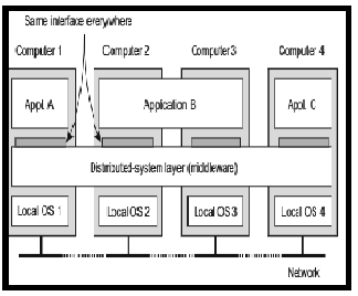
Fig. 1: Distributed system orgnised as a middleware (Source: [2])

By distributing resources to several PCs, networks, or servers, it assists enterprises in managing application or workload requests. Different requests can be fulfilled in this way without jeopardizing the integrity of the system as a whole or its requirements. In order to achieve other load balancing characteristics, such as equitable task distribution among all hosts, facilitation of the quality of service, enhanced system performance overall, shortened response times, and better resource utilization, load balancing is frequently used to prevent bottlenecks. These elements are the most typical check-list items that must be kept in these kinds of apps [5].

Concept of Scheduling and Load Balancing in Distributed Systems

Schedulers are special system software which handles process scheduling in various ways and their major concern is to decide which process is to run and the process to wait. Process Schedulers are of three types [6]:

1. Long-Term Scheduler
2. Short-Term Scheduler
3. Medium-Term Scheduler

The Scheduler selects from among the processes in memory ready to run or execute and the CPU time to one of those processes [6]. Tychalas and Karatza in [7] described Scheduling as fundamental to the success of distributed systems and further stated that even the most powerful high performance computing environments require proper scheduling in order to efficiently serve the users. The techniques used for scheduling the processes in distributed systems are of three distinct types stated following [8].

1. Task Assignment Approach
2. Load Balancing Approach
3. Load Sharing Approach

Basic Concept of Load Balancing

In a Distributed System Environment, distributed scheduling is composed of two parts: local scheduling, (processing resources to jobs within one node – Server), and global scheduling, which determines which jobs are processed by which processor and it is a vital component in any acceptable global scheduling policy [3].  Load balancing aims at improving system performance by even distribution of tasks to processors preventing overload of some processors with work while others remain idle. Jagaty in [9] defined Load balancing as the methodical and efficient distribution of requests across multiple servers. The load balancer sits between client devices and backend servers, receiving and then distributing incoming requests to a server that is healthy and capable of fulfilling them [9]. As a critical component of any distributed system, a load improves the services offered by increasing availability and responsiveness because it distributes the traffic across multiple servers, and also helps us avoiding a single point of failure.

Load balancing plays a vital role in the operation of distributed and parallel computing. It partitioned the incoming workload into smaller tasks that are assigned to computational resources for concurrent execution. The load may be CPU capacity, memory size, network load and delay [4]. The reason behind load balancing is to handle requests of multiple users without degrading the performance of web server. Load balancer receives requests from user, determines the load on available resources, and sends request to the server which is lightly loaded. The major functions of load balancer are [4]:

1. Distributes incoming traffic across multiple computational resources
2. Determines resource availability and reliability for task execution
3. Improves resource utilization
4. Increases client satisfaction
5. Provides fault tolerance and flexible framework by adding or subtracting resources as demand occurs

A technique that benefits networks and resources by offering a maximum throughput with a short response time is load balancing. With load balancing, data may be transferred and received instantly since it distributes the traffic among all servers. The load balancing algorithms’ main objectives are: [10]:

• Cost-effectiveness: Load balancing contributes to lower costs and greater system performance.
• Scalability and flexibility: Over time, the size of the system for which the load balancing techniques are used may change. Thus, the method needs to be scalable and adaptable in order to handle these kinds of scenarios.
• Priority: The tasks or resources that must be completed must be prioritized. Higher priority tasks therefore have a greater likelihood of being completed.

Load Balancing Scheduling Methods

Avanu, in [11] identified and listed four common load balancing scheduling methods with different behavioral characteristics and stated as follows:

1. Least Connections Scheduling (LCS): When using this strategy, the load balancer will route fresh clients to the servers that have the fewest open connections. There will be times when clients are continuously connected to a server, while other servers may amass more client connections than some. One cannot always anticipate a levelling of distribution with load balancing scheduling approaches because when connections come and go or remain connected, certain servers may gain or lose connections more quickly than others. But, the selection of servers to send a client to will continue to be a dynamic decision according to the servers with the Least Connections at the time a client connects.
2. Round Robin (RR): In this approach the load balancer sends client connections to the next available server in a sequential manner. If all connections are equal in duration and activity, it would be reasonable to expect Round Robin to result in the most even distribution of connections to the servers. However, it must be considered that in real world scenarios not all connections will have equal activity and duration.
3. iii. The Weighted Round Robin (WRR): This Scheduling Algorithm is defined as a technique that takes the weight of a node to determine how tasks will be assigned to them.  This technique is an improved version of the RR. It considers using weights assigned to the participating nodes to designate their computational capabilities. For instance, a fixed-powered desktop computer might be given a higher weight than a smartphone with restricted resources, which would be given a lower weight. To ensure that participating nodes with better computing capabilities have more jobs to complete, task distribution is proportionate to each node’s respective weight [12]. As a result, even with Round Robin, certain servers could have more connections than others, especially when clients have a tendency to stay connected for extended periods of time. The Algorithm lists the step-by-step approach for the weighted round-robin algorithm. This algorithm is an improvement of the RR algorithm. In RR, the processing capacity of the processor or VM is not considered while scheduling the task. But in the WRR algorithm, the weight for each VM is calculated based on its processing power. VMs with more processing power have more weight, and VMs
4. Weighted Fastest Response: The Weighted Fastest Response (WFR) scheduling method calculates a value based on the number of current connections, divided by the server weight. It is established that the server with the lowest value is the one that can respond most quickly. Therefore, even with Round Robin, some servers might have more connections than others, particularly in situations where clients frequently stay connected for extended periods of time.

Types of Solutions to the Load Balancing Problem

There are two main approaches depending on whether a load balancing algorithm bases its decisions on the current state of the system or not: Static and Dynamic [3]. In the static approach, priori knowledge about the global status of the distributed system is known and job resource requirement and communication time are assumed.

Hamdan and Marsono in [12]., concluded their work that Static Load Balancing algorithms are simple but costly and only suitable for homogeneous servers, but their inflexible nature makes them unsuitable for dynamic changes. The static algorithm performs load distribution with little or no consideration for the efficiency of the component nodes such as RAM size, server processor, and the link bandwidth. Nevertheless, this algorithm has little overhead with easy implementation, with less overhead and suitable for homogeneous servers [14]. A good example is when more tasks are intermittently sent to the same server without consideration of the server’s ability to handle such task size at the time. Dhinesh and Venkata [15] opined that the decisions related to balancing of load will be made at compile time when resource requirements are estimated. It was emphasized that advantage of Static Load Balancing algorithm is the simplicity with respect to both implementation and overhead, since there is no need to constantly monitor the nodes for performance statistics. Therefore, these algorithms are not well suited for grid and cloud computing environments where the load will be varying at various points of time [13].

In the dynamic approach, there is no a priori knowledge of the current state of the system and therefore load balancing decisions are taken dynamically as shown in Fig. 2. Based on the current state of the system; tasks are allowed to move dynamically from an overloaded node to an under-loaded node to receive faster service [3]. This ability to react to chang es in the system is the main advantage of the dynamic approach to load balancing and finding a dynamic solution is much more complicated than finding a static one and dynamic load balancing produces a better performance because it makes load balancing decisions based on the current load of the system as depicted in Fig. 2.  Dynamic load balancing algorithms use current load information to make changes to the distribution of work load among nodes at run-time and when making distribution decisions [13], [16] and [17]. Dynamic load balancing algorithms are characterized by six (6) policies: initiation, transfer, selection, profitability, location and information [18].

1. Initiation policy: decides who should invoke the load balancing activity.
2. Transfer policy: determines if a node is in a suitable state to participate in load transfer.
3. Selection policy: source node selects most suitable task for migration.
4. Profitability policy: a decision on load balancing is made based on load imbalance factor of the system at that instant.
5. Location policy: decides which nodes are most suitable to share the load.
6. Information policy: provides a mechanism to support load state information exchange between computing nodes.

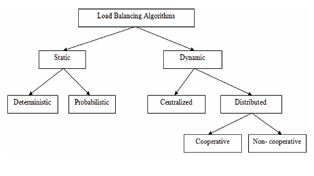
Fig. 2: Load Balancing Approaches- (Adapted – [4])

MATERIALS AND METHODS

The processes of achieving the objective of this research consist of enumerating the major components of a load balancer and the identification of the methods to be used for the development.  The core components of the Load Balancing algorithm are

1. The set of server/servers running the clients on the HDSE

1. • Dynamic Computation of the server weights
   • Dynamic computation of the least connections
2. Load balancer system

The distributed network, there are a number of processors to be responsible for executing the tasks/processes assigned and those tasks are also divided into sub-tasks depending on the number of servers/clients.

The Architecture of the System

The system is based on dynamic algorithm with the combination of two scheduling techniques; the weighted Round Robin (WRR) and the Least Connection (LC) which help the load balancer in the process of decision making on which server to be allocated   the requests based on their current load status (number of requests already allocated). The centralized dynamic load balancing algorithm was implemented in an approach consisting of one server in the HDSE acting as the central server responsible for process allocation to other computing servers (Fig. 3.) Decisions are taken by the central server   based on load information obtained from the other servers in the HDSE.

• assignment of the load was implemented using the

algorithm based on the decision of the load balancer (WRR or LC) for the particular task.

• the steps are repeated for new tasks

The computation of the weight for each VM is carried out dynamically by the associated function and stored in a defined data structure ‘Struct’ along with the Server_ID of the VM (W_variable is a global variable). In accordance with each server’s weight, or preference, new connections are forwarded by the weighted round robin algorithm, which keeps track of a weighted list of servers. This dynamic approach gives nodes additional weight based on their CPU capacity (number of cores) and memory capacity (Algorithm 1) [18], [19], and [20].

For the purpose of this work, the identified server weight properties considered are the number of cores (CPU) and the size of memory. The Linux-like OS (Ubuntu Linux) is the environment for the tests and access to these properties are performed through the following functions; “proc/cpuinfo“ and “getMemorySize (/proc/meminfo”) of the library. The returned values are used to assign appropriate server weights. Each server is identified by its assigned index in the server table.

By sending more requests to the server with the highest capacity, it benefits the algorithm. Weighted RR distributes requests to the node in a cyclical manner, just as RR. Nodes with higher specs receive more attention from the load balancer. The Least Connection (LC) is equally computed dynamically using a global variable defining the identified Server_ID and the N_connect for the number of connections (Algorithm 5).  After the assignment of a task (the function is triggered) to a VM the N_connect of the variable of the VM is incremented and decremented after completion of the task (equally triggered).

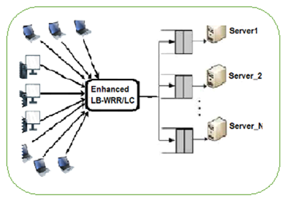
Fig. 3. Architecture of the Load Balancer

Load Balancing Performance Metrics

Performance metrics (numerical values) are often used to measure the state of the load balancers and illuminate areas of improvement [21].  The Response time, waiting time and the Throughput were considered in this paper.

• Throughput

Throughput is the measurement of a successfully completed job which, in the case of the load balancer, means the number of requests successfully completed per unit time. This is an insightful metric to measure since higher throughput indicates higher efficiency of your load balancers, signalling healthy load balancing.

• Response time

Response time is the time algorithms take to respond to a request. This includes a sum total of waiting time, transmission time, and service time that the system requires.

•  Waiting time

  Waiting time is the total time spent by the

   process in the ready state waiting for CPU.

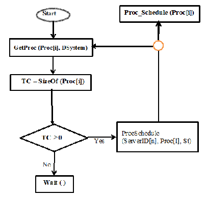
Fig. 4. Flowchart for the Allocation of Processes Based on Completion Time (CT)

Steps for the Scheduling Process

Based on the output of the flowchart, the returned value of the time complexity will be the input of the next step with the server identity; S_id. The next step will be to determine the state of the server (the current policy) and other related information before deciding how and type of the policy that will be implemented. The WRR and LC policies are considered in this work. The algorithm will return the expected completion time of Proc[i] and the S_id will be used to determine the approximate weight value of the node.

Designing the Algorithm – (Check Servers without assigned weight value)

The next step is to compute the load of the Server with the returned value time complexity TC of the participating servers, hence. The ratio of each Server’s actual connections and weight are computed and then the task is assigned to the server with the least ratio and least completion time.

Performance evaluation test

The test was carried out on a DELL Server running Ubuntu 12 version with the necessary tools to create VMs.

The developed load balancing algorithm with varying capacities in an HDSE was tested, and the results showed that this approach performed marginally better than other load balancing algorithms currently in use. Instead of using the developed dynamic technique, the majority of current LBAs allocate server weights in a fixed manner. The goal of an HDSE’s load balancing algorithms is to constantly adjust parallel program response times by fine-tuning the process scheduling strategies on individual machines. It should be noted, nevertheless, that due to a few intrinsic limitations, dynamic programming is not so simple [23]. Studies have indicated that load balancing has not fully benefited from the use of static and dynamic variables. Hybrid algorithms could then grow. In an effort to get around the drawbacks of both algorithms, hybrid approaches combine the best aspects of static and dynamic load balancing strategies [24].

Some of the necessary schemes are illustrated in Algorithms 1 – 5.

Algorithm 1: Scheduling Algorithm (Weight/Alloc)

    Int N = 0 ; Initialisation

Int ServerTable [16]

; Initialisation Max servers = 32

While N++ > 0 and N <  Num_nodes

; Scan through all the servers of the HDSE

; If there is any node in the HDSE

where ꟽᵢ < 1

; Skip the node and compute the Server weight

; Insert the Node_id  in  the table  of Servers

; record the weight of the node

Else

    Server_ID.W_variable = computeweight (Server_ID)

; Assign a ꟽᵢ to the Server

End If

End While

Algorithm 2:  The Load balancing Algorithm

n_task ;  number of tasks to be sent between processes

{

Prj_Algo Init (&argc, &argv); //Initializing Main program  Func_Value (ProcSchedule (S_id[n], Proc[i]),&request)

(

// Determine TC of process, Weight

If  T_C  > 0 and ꟽᵢ  > 0 then

Process_Task()

else

End IF ; skip

return (Func_Value)

}

return Server_ID[i];

}

Algorithm 3: Compute_StartTime ()

; This algorithm computes the start time of the process in millisecond and

// returns the result to the calling function.

Function StartTime ( )

{

gettimeofday (&tv,&tz);   // in-built Function Linux

tm = localtime (&tv.tv sec); // Time of the day

starttime  = tm.tm-hour * 3600 * 1000 + tm.tm.min

* 60 * 1000 + tm.tm-sec * 1000 + tv.tv usec / 1000;

Return (starttime);

}

Algorithm 4: Task Stop Time Computation

ComputeStop_Time (starttime, Task[i])

; This algorithm Computes the stop time of each of the node process

; starttime variable contains the start time earlier computed  and the

; Task[i] of the process

{

startt = starttime;

gettimeofday(&tv,&tz);

tm = localtime(&tv.tv sec); // a data structure

stopp = tm¿tm hour * 3600 * 1000 + tm.tm min * 60 * 1000 +tm.tm

sec * 1000 + tv.tv usec / 1000;

return (Task[i], stopp – startt);

exit (stop);

}

Algorithm 5: Computation of LC

Compute_LC (Server_Id.Task[id])

{

; Check if Task[i] has just been assigned/active

If (Server_Id.Task[id])

++Server_Id .N_connect

else

–Server_Id .N_connect

Return 1;

}

Turn Around Time (TAT)

TAT = ComputeStop_Time (starttime, Proc[i]) – StartTime (starttime, Proc[i] )                                                                    (1)

RESULTS AND DISCUSSION

TABLE I: Output of the ld_balancer with 8 Virtual Servers (Millisecs)

PID	S_ID	BTime	WTime	TATime
11200	1	8	0	8
10230	2	4	12	16
11209	3	8	16	24
12345	4	12	24	36
13456	5	3	22	25
11201	6	6	10	16
14567	7	8	6	14
17235	8	2	8	10

TABLE 2: Output of the ld_balancer with 8 Nodes (Millisecs) CT = Stop time – Start time

#	PID	S_Id	CT
1	11200	1	4
2	10230	2	6
3	11209	3	8
4	12345	4	10
5	13456	5	8
6	11201	6	12
7	14567	7	6
8	17235	8	8

Values TAT, WTime and THP

• Average TAT: 98/8 = 18.62 (milliseconds)
• Average waiting time (WTime) = 12.25 (milliseconds)
• Throughput (THP) – Process total time of completion.
• Average Process Completion Time = Starting Time – End time
• THP = 62 / 8 = 7.75 (milliseconds)

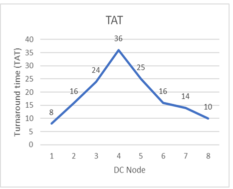
Fig. 5: Graph showing the TAT for each server 8-Processes

DISCUSSIONS

The TAT was plotted against the server_ID for the computation of the TAT. While the average TAT is 18.62milliseconds for eight nodes, the average waiting time is 12.65 milliseconds reasonably compared with other conventional Load balancer on Heterogeneous DSE. A very important observation however is the fact that, the TAT peaked on server number four (4) for the possible reason of the weight of the server which was readily high. The TAT increases as the weight (ꟽ) of the server increases. Process (PID) 12345 has the highest waiting time (see Table 1) as a result of the time usage by the processor (due in part to the processor time).

CONCLUSIONS

An enhanced algorithm for a load balancer in a Heterogeneous DSE that has proved to be effective in terms of performance and a higher accuracy level needed in such an environment has been successfully developed. The description of the main features of load balancing algorithms has been elicited and carried out considering the requirements of this work. A review of related works of different load balancing algorithms and test of the efficiency indicators are also indicated.

Scalability of the developed Algorithm

The developed algorithm was first tested with 32 VMs and  the inconsistency in the response time was observed with other parameters stable. However, when lowered (16), the response time improved along with the TAT. The amount of memory was discovered to be responsible and have decided to improve on the memory capacity of the LBA Server.

Constraints

The authors have experienced no serious constraints except in the provision of additional hardware components for the server. The authors hope for some interventions on funding.

Future Work Direction

The project is still ongoing as other parameters are expected to be included in the dynamic computation of weights for a newly introduced client-server. Inclusion of disk capacity, speed, bandwidth, table of weights (Lower and Upper bound) and fault tolerant are  to be improved upon

REFERENCES

1. Lindsay, D., Gill, S.S., Smirnova, D. et al. (2021). The evolution of distributed computing systems: from fundamental to new frontiers. Computing 103, 1859–1878 (2021). Available at:  https://doi.org/10.1007/s00607-020-00900-y
2. Marten van Steen, Maarten and Tanenbaum, Andrew. (2016). A brief introduction to distributed systems. Computing. 98. 10.1007/s00607-016-0508-7.Available at:https://www.researchgate.net/publication/306241722A_brief_introduction_to_distributed_systems
3. Ali M. Alakeel (2010). A Guide to Dynamic Load Balancing in Distributed Computer Systems. Intl. Journal of computer science and Network Security http://paper.ijcsns.org/07_book/201006/20100619.pdf
4. Shukla, A., Kumar S. and, Sing, H. (2020). Analysis of Effective Load Balancing Techniques in Distributed Environment. 10.5772/intechopen.91460.
5. Nageswara Prasadhu N. (2020). An Efficient Hybrid Load Balancing Algorithm for Heterogeneous Data Centers in Cloud Computing June 2020 International Journal of Advanced Trends in Computer Science and Engineering 9(3):3078-3085. DOI: 10.30534/ijatcse/2020/89932020
6. Jeerry Breecher (2021). Operating System Scheduling. https://web.cs.wpi.edu/~cs3013/c07/lectures/Section05-Scheduling.pdf
7. Dimitrios Tychalas and Helen Karatza (2020). A Scheduling Algorithm for a Fog Computing System with Bag-of-Tasks Jobs: Simulation and Performance Evaluation. Elsevier Publisher. https://doi.org/10.1016/j.simpat.2019.101982.
8. Srivastava, S. and Banicescu, I. (2018). Scheduling in Parallel and Distributed Computing Systems. In: Prasad, S., Gupta, A., Rosenberg, A., Sussman, A., Weems, C. (eds) Topics in Parallel and Distributed Computing. Springer, Cham. https://doi.org/10.1007/978-3-319-93109-8_11
9. Pratyush Jagaty (2023). Load Balancing in Distributed Systems. Available at: https://system.camp/tutorial/load-balancing-in-distributed-systems/
10. Igor N. Ivanisenko and Tamara A. Radivilova (2019) Survey of Major Load Balancing Algorithms in Distributed System. Available at: https://arxiv.org/ftp/arxiv/papers/1904/1904.05923.pdf
11. Avanu (2020). Load Balancing Scheduling Methods Available at: https://avanu.com/load-balancing-scheduling-methods/.
12. V., Mohamudally, N. and Nissanke, N. (2020), A Dynamic Load Balancing Algorithm for Distributing Mobile Codes in Multi-Applications and Multi-Hosts Environment. Published in the International Journal of Computer Science Issues, Vol 17, Issue 4, July 2020 www.ijcsi.org DOI: 10.5281/zenodo.3991567
13. Ranjit Rajak, Anjali Mohammad and Sajid Mohammad (2023). Load balancing techniques in cloud platform: A systematic study. DOI: 10.52756/ijerr.2023.v30.002 https://www.researchgate.net/publication/370482519_Load_balancing_techniques_in_cloud_platform_A_systematic_study
14. Mosab Hamdan and M.N. Marsono (2021). A comprehensive survey of load balancing techniques in software-defined network – Static algorithms for server load balancing. Journal of Network and Computer Applications, 2021. https://www.sciencedirect.com/topics/computerscience/static-load-balancing
15. Dhinesh B. and Venkata K. (2013). Honey bee behavior inspired load balancing of tasks in cloud computing environments. Elsevier B.V. All rights reserved. http://dx.doi.org/10.1016/j.asoc.2013.01.025
16. Bibhudatta Sahoo, Dilip Kumar and Sanjay Kumar Jena (2012). Observing the Performance of Greedy algorithms for dynamic load balancing in Heterogeneous Distributed Computing. Available at: https://www.researchgate.net/publication/259810449_Observing_the_Performance_of_Greedy_algorithms_for_dynamic_load_balancing_in_Heterogeneous_Distributed_Computing_System
17. Mahdi S. Almhanna, Tariq A. Murshedi, Firas S. Al-Turaihi et al. (2023). Dynamic Weight Assignment with Least Connection Approach for Enhanced Load Balancing in Distributed Systems, 07 August 2023, PREPRINT (Version 1) available at Research Square [https://doi.org/10.21203/rs.3.rs-3216549/v1]. (Accessed 26 Dec. 2023)
18. Educative (2023) What is the least connections load balancing technique? Available at:https://www.educative.io/answers/what-is-the-least-connections-load-balancing-technique (Accessed 14 Dec 2023)
19. IBM (2023) Weighted round robin. Available at: https://www.ibm.com/docs/en/datapower-gateway/10.0.1?topic=groups-algorithms-making-load-balancing-decisions#lbg_algorithms__wrr. (Accessed 14 Dec 2-23).
20. Array (2021). Load Balancing Metrics https: //arraynetworks.com/load-balancer-important-metrics-impacting-performance/System
21. Mohamed Hanine and El-Habib Benlahmar (2020). A Load-Balancing Approach Using an Improved Simulated Annealing Algorithm. Journal of Information Processing Systems ISSN: 2092-805XVolume 16, No 1 (2020), pp. 132 – 144, 10.3745/JIPS.01.0050
22. Chang, T., Xin, T., Hu, L., & Xiong, W. (2021). Dynamic weight load-balancing method of cloud-center based on Nginx. Journal of Chongqing University of Posts and Telecommunications: Natural Science Edition, 33(6), 991-998
23. Igor N. Ivanisenko and Tamara A. Radivilova (2019) Survey of Major Load Balancing Algorithms in Distributed System.  Available at: https://arxiv.org/ftp/arxiv/papers/1904/1904.05923.pdf
24. Chukwuneke, Chiamaka Ijeoma; Inyiama, Hyacinth C.; Amaefule, Samuel; Onyesolu, Moses Okechukwu and Asogwa, Doris Chinedu (2019). Review of Hybrid Load Balancing Algorithms in Cloud Computing Environment. International Journal of Trend in Research and Development, Volume 6(6), ISSN: 2394-9333 www.ijtrd.com. Pg. 31-37.