
Exploring Dimensionality Reduction Techniques for Improved Breast Cancer Diagnosis
- Akampurira Paul
- Mutebi Joe
- Mugisha Brian
- Muhaise Hussein
- Kyomuhangi Rosette
- 808-824
- Jun 14, 2024
- Health
Exploring Dimensionality Reduction Techniques for Improved Breast Cancer Diagnosis
Akampurira Paul, Mutebi Joe, Mugisha Brian, Muhaise Hussein, Kyomuhangi Rosette
Kampala International University, Uganda
DOI: https://doi.org/10.51244/IJRSI.2024.1105051
Received: 20 April 2024; Revised: 06 May 2024; Accepted: 10 May 2024; Published: 14 June 2024
ABSTRACT
A crucial area of medical study is the diagnosis of breast cancer, where managing the inherent complexity of high-dimensional information poses a challenge in addition to precise identification. In order to improve diagnostic accuracy, this research investigates dimensionality reduction strategies. This study’s main goal was to improve the accuracy and interpret ability of breast cancer diagnosis by using dimensionality reduction techniques. The goal of the study is to find significant patterns for useful diagnostic models by examining how preprocessing methods affect a high-dimensional dataset. Starting with a dataset including 569 observations and 30 attributes, careful examination reveals imbalances in the dataset (63% benign, 37% malignant). We used Pearson correlation coefficients to detect and eliminate highly correlated features in order to address multi collinearity. A subsequent adjustment of the data using min-max normalization guarantees consistent weighting. Then, for thorough dimensionality reduction, Principal Component Analysis (PCA) is employed. Screep lots and biplots are used to visually represent data, highlighting how well-suited early principle components are for separating benign from malignant instances. Our findings confirm the effectiveness of the procedure by showing a significant 24% decrease in data dimensionality. This work highlights the critical role that dimensionality reduction plays in improving breast cancer diagnosis for more precise, effective, and understandable models, and it calls for further investigation of the specific findings.
Keywords: Breast cancer, high-dimensional datasets, early diagnosis, dimension ality reduction, machine learning, artificial intelligence.
INTRODUCTION
An estimated 9.6 million people died from cancer in 2018, making it the second highest cause of death worldwide. Breast cancer alone accounts for about 2.09 million fatalities per year, with a startling 70% of these deaths occurring in low- and middle-income nations (IARC, 2018; WHO, 2021). Given that breast cancer accounts for 25% of all cancer incidences in women, its prevalence highlights the critical necessity to address the disease (Bray F, 2022). Even though it is highly prevalent, late-stage presentations, difficult-to-get diagnoses, and few treatment choices are still present, especially in low-income nations, making it even more of a global health concern (Wilkinson L, 2022). According to recent estimates of the global cancer burden, 2.26 million incident cases of breast cancer are expected to occur in 2020, making it the primary cause of cancer-related death for women globally. Interestingly, there is a strong correlation between the incidence of breast cancer and human development. Areas experiencing economic transition are predicted to see a notable increase in the number of cases. However, survival rates are still much lower in less developed areas, which can be related to things like access to adequate treatment and delays in diagnosis (Huang J, 2021).
The International Agency for Research on Cancer (IARC) reports that Uganda has a notable cancer incidence. 320 newly diagnosed cases are reported for every 100,000 individual s1. An estimated 200,000 instances, both new and old, including those that have been treated and cured, exist at any one time 1. Regretfully, 80 out of every 100 newly diagnosed cases end in death (IARC, 2022).
The fact that 30% of cancer cases are treatable if detected early emphasizes the vital need for early detection measures. The late diagnosis rate makes the fatality rate worse. In order to promote early-stage identification, early diagnosis initiatives are essential. They do this by improving access to breast cancer therapy and efficient diagnostic services. (Tobore, 2019)
Breast cancer is a worldwide health emergency that has to be addressed immediately, especially in low- and middle-income nations. This highlights the vital need for creative and effective diagnostic techniques. Millions of people die from breast cancer every year, making it a deadly and widespread illness that calls for a deliberate change in diagnostic approaches. The need for revolutionary solutions is increased by the high incidence of breast cancer, which accounts for a sizable fraction of all cancer cases among women. It is also compounded by ongoing issues such as late-stage presentations and limited access to effective diagnosis and treatment. (Wilkinson L, 2022).
Classifying malignant and benign malignancies is a critical function of computer-aided diagnostic (CAD) systems, which also improve physician performance by decreasing misdiagnoses and diagnosis times. (Chhatwal J, 2010). Using a variety of classification techniques, machine learning (ML), a subset of artificial intelligence, has been widely used in cancer diagnosis and detection. Notwithstanding advances in technology, problems still exist, particularly in low-income nations. When combined with Electronic Medical Records (EMRs), artificial intelligence (AI) has the potential to revolutionize healthcare services.(Bekbolatova, 2024).Understudied, nevertheless, are ML’s effectiveness and applicability in low-resource environments, such as low-income nations. It is clear that effective diagnosis tools are needed in settings with limited resources, and AI applications like Natural Language Processing (NLP) are already helping to guide cancer treatments.(Shastry, 2022). The contextual background highlights the need for effective and precise diagnostic tools in a variety of scenarios while acknowledging the promise of machine learning to transform healthcare delivery. (Katarzyna Kolasa, 2023).
Additionally, a new method called ensemble learning combines several classifiers to enhance predictive performance. (Habehh, 2021)
High-dimensional datasets present problems for breast cancer diagnosis, requiring sophisticated methodologies for efficient model construction.
The myriad of characteristics that go into determining whether a breast cancer is malignant or benign makes diagnosis more difficult (Iqbal, 2022). Accurately reporting the facts is hampered by human interpretation, which is frequently subjective and based on personal experience, particularly when the number of samples rises.
The use of CAD systems and ML shows potential against the backdrop of the growing burden of breast cancer.Additionally, a new method called ensemble learning combines several classifiers to enhance predictive performance.High-dimensional datasets present problems for breast cancer diagnosis, requiring sophisticated methodologies for efficient model construction.
The myriad of characteristics that go into determining whether a breast cancer is malignant or benign makes diagnosis more difficult (Iqbal, 2022). Accurately reporting the facts is hampered by human interpretation, which is frequently subjective and based on personal experience, particularly when the number of samples rises.
The use of CAD systems and ML shows potential against the backdrop of the growing burden of breast cancer.Additionally, a new method called ensemble learning combines several classifiers to enhance predictive performance. (Farrell S, 2022; Cao, 2019).
In addition to taxing computing power, high-dimensional datasets run the danger of adding noise and extraneous characteristics, which could reduce the precision of diagnostic models (Thudumu, 2020). Reducing dimensionality makes the most informative information more visible, which improves the diagnostic process’s effectiveness and interpret ability. Because dimensionality reduction might potentially address late-stage presentations and limited accessibility to appropriate diagnosis, especially in situations with limited resources, its significance is increased. (Jia, 2022).Diagnostic models that are more effective, precise, and easily comprehensible can be achieved through the use of dimensionality reduction techniques, which simplify datasets and reveal significant patterns. Investigating these methods is in line with artificial intelligence’s revolutionary potential to change the way healthcare is delivered.(Vogelstein, 2021).
Thus, in order to determine the inherent value of dimensionality reduction strategies for breast cancer diagnosis, our study started with practical experimentation.
MATERIALS AND METHODS
Dataset:
The study utilized the Wisconsin Breast Cancer Database (WBCD) dataset which has been widely used in research experiments. R Studio was used for the entire data preparation, analysis and modeling. The WBCD dataset for breast cancer diagnosis is comprised of feature values calculated from digitized image of a Fine Needle Aspirate (FNA) of a breast mass. These features describe the characteristics of the cell nuclei present in the image. This database is also available through the UW CS ftp server: ftp ftp.cs.wisc.edu cd math-prog/cpo-dataset/machine-learn/WDBC. This standard dataset is suggested for use in data science and machine learning experiments and is accessible to the public.
Several attributes make up the data, such as the ID number, the diagnosis (M = malignant, B = benign), and For every cell nucleus, ten real-valued characteristics are computed: radius (mean of distances from center to points on the perimeter), texture (standard deviation of gray-scale values), perimeter, area, smoothness (local variation in radius lengths), compactness (perimeter^2 / area – 1.0), concavity (severity of concave portions of the contour), concave points (number of concave portions of the contour) and symmetry, fractal dimension (“coastline approximation” – 1).
For every image, the mean, standard error, and “worst” or biggest feature (mean of the three largest values) of these features were also calculated, yielding a total of 30 features. Radius SE is found in field 13, mean radius is found in field 3, and worst radius is found in field 23.All feature values are recoded with four significant digits.
The downloaded dataset was loaded and saved into the R integrated development environment (IDE), R Studio. This professional data science software is suitable for enterprise use and offers free and open-source tools for statistical modeling and R programming.
To have a look at our data, we used the function view() to glance at our data as follows.
Table 1: Data import view in R studio
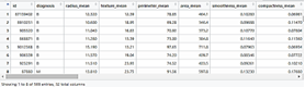
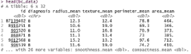
A quick look at the imported data (Table 1) revealed that there are 569 rows of instances and 32 columns of features (variables) in our data. Since none of the variables had spaces in their names—a naming strategy that would have made them incompatible with several of the R functions we would use—our data was quite clean. We also looked at the structure of the data by using head(), which also show a detailed view of the data in terms of data structures of the features, as follows;
Table 2: data head view
Data Pre processing:
In order to deal with the multicollin earity problem, highly correlated characteristics were identified and removed using Pearson correlation coefficients. This procedural step played a crucial role in strengthening the robustness of the studies that followed. After the correlation analysis, min-max normalization was applied to guarantee that features were weighted consistently, reducing the influence of different scales on the model-building procedure.
Outlier detection (neutralization and or removal):
Anomalies or numbers that differ from the average when compared to the bulk of observations are known as outliers. These non-representative samples, which are usually the result of measurement errors, coding problems, or occasionally naturally occurring anomalous values, have a significant impact on the results of subsequent models. As such, a thorough analysis of the data was carried out in order to detect and eliminate outliers based on their relative significance.
Dealing with missing data
The simplest solution to deal with missing data is to reduce the size of the dataset by eliminating those samples that have insufficient values. This method works especially well for large datasets if the percentage of missing values is small compared to the whole dataset. On the other hand, if the researcher decides not to reject samples that have missing values, then efforts need to be taken to impute appropriate values in their place.
The findings indicated that there was no missing data in our data collection, as seen below. We used the is.na function of x to find missing values and return the total number of missing values for each variable.
map in t(bc data, function(.x) sum(is. na(.x)))
| diagnosis | radius mean | texture mean | perimeter mean |
| 0 | 0 | 0 | 0 |
| area mean | smoothness mean | compactness mean | concavity mean |
| 0 | 0 | 0 | 0 |
| points mean | symmetry mean | dimension mean | radius se |
| 0 | 0 | 0 | 0 |
| texture se | perimeter se | area se | smooth ness se |
| 0 | 0 | 0 | 0 |
| compactness se | concavity se | points se | symmetry se |
| 0 | 0 | 0 | 0 |
| dimension se | radius worst | texture worst | perimeter worst |
| 0 | 0 | 0 | 0 |
| area worst | smoothness worst | compactness worst | concavity worst |
| 0 | 0 | 0 | 0 |
| points worst | symmetry worst | dimension worst | |
| 0 | 0 | 0 |
Since there are no missing observations in our data frame, as can be seen from the above, we moved on to data normalization.
Normalization
Diverse methodologies exist for normalizing data, encompassing decimal scaling, Min-Max normalization, and Z-score normalization. In this study, the former was employed due to its compatibility with a majority of algorithms involved in the normalization process. We applied the min-max normalization which would transform a feature such that all of its values fall in range between 0 and We applied min-max normalization as follows;
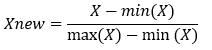
In essence, the formula takes the minimum value of X and divides it by the range of X for each value of feature X. The resultant normalized feature values can be understood as representing the original value’s range between the original and maximum, from 0% to 100%.
Data reduction (Feature selection and extraction)
In order to determine each feature’s importance in connection to the target variable or result and how they interrelate, the researcher dug further into the dataset during this phase. Highly associated features were carefully handled, features judged insignificant were removed, and collinearity tests were carried out. The standardized approach of Principal Component Analysis (PCA), a flexible technique for lowering data dimensionality and improving feature selection criteria, was also used to reduce dimensional space.
Although there are a number of approaches for reducing dimensionality, including the relief algorithm, entropy-based feature ranking, Chi Merge, value reduction, and case reduction, the researcher chose Principal Component Analysis (PCA) for this study because of its simple yet thorough techniques. PCA serves as a method to transform the initial dataset, represented by vector samples, into a new set of vector samples with derived dimensions as shown in the results sub-section.
RESULTS
According to the results presented in Table 2, the majority of the data attributes were stored in double-precision floating-point (dbl) and character (chr) formats. The dataset consists of an extensive 32-column array with 569 elements or instances. A ‘id’ column and labels indicating the goal values as ‘B’ for Benign and ‘M’ for Malignant are among these. In order to get the data ready for analysis and visualization, preprocessing steps included relocating features (columns), reordering them, deleting characteristics like “id,” and substituting full names for diagnosis labels.
Table 3: diagnosis label redefined
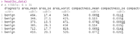
Next, we eliminated the features—like the ID variable—that are in no way required for modeling the data. We saw that the labels for the target variable, malignant or non-cancerous, were m and b, respectively. Additionally, we require the whole names of the diagnosis fields for the data to be easily understood. As a result, we have revised the labels for benign and malignant conditions in Table 3. Following the first round of preprocessing, a raw count of the data reveals 569 observations and 30 features or predictors. Additionally, we found that there are no missing values and that all of the predictors contain continuous values for observations. We observed that every observation was documented as a series of decimal numbers. We took a quick count through our dataset to verify the number of examples and the categories where they belong as follows;
Table 4: cancer rate count
| benign | malignant |
| 357 | 212 |
The target variable for diagnosis, which might be either benign or malignant, is displayed in Table 4 above. According to the tables, 357 of the 569 observations were benign or non-cancerous, while 212 were malignant or cancerous. We further verified that our response (target) variable was balanced using the percentages shown in Table 5;
Table 5: Response carri able
| benign | malignant |
| 63 | 37 |
Table 5 above demonstrates that only 37% of the total dataset has a response variable that leans toward benign or malignant. This indicated that malignant cells were found in 37% of the patients. As a result, the balance check reveals that the data is somewhat off. Table 5 above demonstrates that only 37% of the total dataset has a response variable that leans toward benign or malignant. This indicated that malignant cells were found in 37% of the patients. As a result, the balance check reveals that the data is somewhat off.
Checking for multi collinearity
An analysis of multicollinearity was conducted to find any link between the variables. In order for an analysis to be considered robust, most machine learning algorithms need that the predictor variables be independent of one another. For this reason, the researcher conducted an analysis that resulted in the detection and elimination of multicollinearity. To look for connections between the features in our dataset, we employed Pearson correlation. Mathematically, the two random variables x and y’s Pearson correlation coefficient (ρ) is represented as follows:
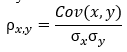
where Cov (x y), is the covariance of x; y, σx is the standard deviation of x; and σy is the standard deviation of y. In R, the cor() function performs the above as follows;
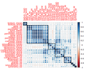
Fig 1: Visualizing correlations with corrplot
The correlation strength, or the absolute value of the correlation coefficient between two variables, is indicated by the circle’s dimensions and color intensity in figure 1, above. Correlates that are positive are colored blue, and those that are negative are colored red. The association between concavity worst and points worst, among other examples, in the graphical representation highlights the presence of correlated variables, all of which were addressed in later procedural phases.
The graphical representation in figure 2 attests to the presence of correlated variables. Pearson correlation coefficients, ranging from -1 to 1, reveal that any feature registering a value of 0.9 or higher in our visual representation signifies a remarkably robust positive correlation. Conversely, features with values of -0.9 or lower denote a pronounced negative correlation, necessitating their exclusion for enhanced model efficacy. Noteworthy examples of highly positively correlated features encompass Area se, texture mean, and texture worst. The ensuing step delineates the methodology employed by the researcher to scrutinize highly correlated values through the utilization of the caret package.
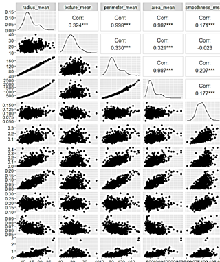
Figure 2: Correlation Plots for Dataset Features.
Checking for multicollinearity among the features
As shown in the figure 2 above, correlation analysis, a detailed clarification of the relationships between the features was obtained. The correlation coefficients indicated how much some features are highly dependent on one another, which could undermine the stability of our modeling results. As a result, this made it easier for the researcher to find and then reduce these correlations, which were best illustrated by characteristics like area mean and radius mean. In order to tackle this, the investigator chose to apply principal component analysis, a method that is discussed in the parts that follow. Before exploring this analytical method, a more thorough analysis of correlations was carried out with the help of scatter diagrams, as described in figure 2.
The correlation plots’ visual portrayal provided information about the relationships between various features. It is crucial to emphasize that correlation, as it is presented here, is not the same as causation; rather, it is a descriptive measure of observed relationships. Notable trends surfaced, explaining a strong positive association between the perimeter, area, and radius means. Furthermore, favorable relationships were found between the radius mean and the concavity mean and the compactness mean. The intrinsic skewness in the data was clarified by the scatter diagrams, which also disclosed the distributional properties of the features.
The researcher used the find correlation() function from the caret package to try to lessen the effect of strongly linked predictors. This function routinely found variables for elimination with a Pearson’s correlation coefficient equal to or greater than 0.9 by using a heuristic technique. The function to remove characteristics with such high correlations was then run by the researcher, and a refined dataset known as bc data corr 1 was produced.
bc data corr 1 <- wisc bc data%>% select(-find Correlation (bc data, cutoff = 0.9)). >ncol(bc data corr 1)
[1] 22.
The resulting dataset from the above transformation is 10 variables shorter and is only comprised of 22 predictors in the dataset bc data Corr1.
Normalizing our data
An important step that the researcher conducted was data normalization, which is a crucial process that is mostly carried out to reduce bias resulting from the scale-related discrepancy in the relative importance of absolute values and their relative equivalents. In order to give each variable equal weight throughout the modeling phase, the normalization technique was essential in establishing parity among the variables.
By utilizing the min-max normalization technique, we methodically modified a feature so that its values were limited to the range of 0 to 1. A feature’s normalization followed the following formula:
![]()
Essentially, the formula operates on each instance of feature X, subtracting the minimum X value and subsequently dividing by the range of X. The resultant normalized feature values can be construed as denoting the percentage distance, ranging from 0 to 100, at which the original value is positioned within the spectrum between the minimum and maximum values. In order to put our data on a consistent scale, a normalizing function was created. Then, this normalization function, which is represented by the notation “normalize(),” was used on columns 2 through 30 of the bc_data data frame (without including the diagnostic variable). The variable bc_data_norm was then given the output once it had been transformed into a data frame. The suffix “_norm” is only used as a memory aid to emphasize that the values in the dataset have been normalized. This approach promoted fair variable treatment, strengthened the modeling process’s resilience, and made it easier to establish a uniform framework.
Dimensionality reduction through Principal component analysis
Dimensionality reduction is an intricate process that involves reducing the size of a dataset’s feature space, or dimensions, in preparation for model training (Jia, 2022). The primary goal of the investigator’s dimensionality reduction effort was to reduce the amount of time and storage needed for data processing. This project aimed to improve model inter pretability, boost data visualization, and avoid the negative consequences of the dimensionality curse. Essentially, the goal was to remove redundant and unnecessary data in order to save computing expenses and reduce the possibility of over fitting. The two main techniques involved in this endeavor are feature extraction and feature selection.
When it comes to feature selection, a subset of variables is carefully selected to produce a basic set of features that are devoid of unnecessary or redundant characteristics and may be eliminated without materially affecting the performance of the model. The variable ‘id’ was removed in this case because the modeling method did not consider it relevant. Although there are other approaches, like the feature selection method, that might eliminate less significant characteristics, we purposefully decided not to remove any more features from our dataset.
Given that some associated yet informative features might be eliminated using the feature selection approach, the researcher was faced with the need to combine these correlated features into a single entity using the feature extraction method. Feature extraction, also known as feature projection, is the process of converting high-dimensional data into lower dimensions by means of mathematical functions so that the newly extracted features take the place of the originals. Principal Component Analysis (PCA) is the gold standard methodology for extracting such bright features.
As previously explained, principal component analysis (PCA) is a linear feature extraction method that functions in a low-dimensional space to distinguish data that was initially stored in a high-dimensional environment. With the use of this technique, the researcher was able to carry out an analysis that would allow the data to be mapped onto a lower dimension, maximizing the variance of the data in its low-dimensional representation. PCA was the method of choice because of its unmatched effectiveness when datasets have an abundance of features along with inter-feature redundancy or correlationa situation supported by our previous study of multicollinearity in the dataset.As a result, to eliminate redundant features, high-dimensional data were transformed into lower dimensions using principal component analysis (PCA), which effectively captured most of the variance present in the original features.
The process was done using the following steps;
- Finding the mean vector
 where indicates the data points and n denotes the number of points,
 - Computing the covariance matrix

- Computing the eigenvectors, φ, and the corresponding eigenvalues.
- Ranking and choosing the top k eigenvectors.
- Construct a n x k dimensional eigenvector matrix, U. Here the n, is the number of original dimensions and k is number of eigenvectors. And
- Transform the data samples to new subspace in the equation

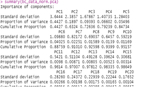
Summary of the PCA results
Table 6, shows a summary of the PCA implementation results and 84.73% of the variance is explained by the first five PC’s and the first 15 components explain 98.64% of the variance as in table 6.
Table 6: Summary of PCS results
Importance of components and Eigen values using covariance matrix
We used the predict function to output the values of the principal components: Get the eigen values of correlation matrix which further show the importance of components.
Table 7: Eigen values using covariance matrix
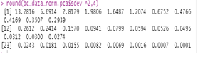
From the table 7, the components that have small eigenvalues show very little variation and their influence on the target prediction or the outcome values from the diagnosis is thus minimal. We further visualize the principal to explicitly understand the component importance using a screeplot as follows;
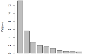
Fig 3: screeplot to visualize the relative importance of principal components
The eigenvalue, represented by the y-axis in the screeplot above, indicates the major components’ relative importance. The first ten main components and how they helped forecast the target variable are depicted in the picture. We used biplots to provide a thorough picture in order to better grasp this. We utilized biplot, which depicts data and the projections of original features, to determine how variables and data are mapped with respect to the principal component. Figure 4 demonstrates how successfully the first two components were able to distinguish the diagnosis. PC1 has a bigger impact on determining whether a tumor is benign or malignant. However, we would need a more thorough examination of the factors that affect the first two components the most. We also aimed to clarify the distinction between benign and malignant tumors. In order to try to make more sense of the figure, we added the response variable (diagnosis):
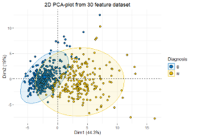
Fig 4: First 2 PCA features
The initial pair of components conspicuously reveals a discernible demarcation between benign and malignant tumors. This unequivocally signals the aptness of the data for a classification model, such as discriminant analysis. The distinct separation observed between the ‘Malignant’ and ‘Benign’ categories, based on approximately 63% of variance in a 30-dimensional dataset, underscores the potential efficacy of utilizing merely two dimensions in a plot. While these dimensions may yield reasonably accurate estimates, grappling with higher-dimensional data proves challenging yet concurrently encapsulates a greater extent of variability.
Interestingly, we find that more than 60% of the variance can be explained using just the first two factors. The variance of each variable from its average is explained by representing the variables as vectors or arrows, where the origin represents the mean value and the data points or sample identifiers indicate the scores. The centroid of the data matrix is, interestingly, the average, which is placed at zero. The arrows’ lengths provide a proportionate representation of variability by directly correlated with it.
The angle at which two arrows are oriented indicates the degree of correlation between the variables; sharp angles indicate strong positive correlations, while more obtuse angles indicate negative correlations. In order to explore these interactions further, corrplots—which show the component variability trajectory visually—were used. The following graphic explains the importance of each variable in the overall analysis.
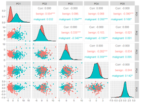
Fig 5: a correlation plot of the first five principal components
The aforementioned graphic illustrates the use of PCA to assess component relevance by removing strongly correlated variables from the bc data corr1 dataset. The outcomes demonstrate how well the first component handles the data. The components from PC2 to PC5 become less significant as we proceed.
PCA Using our normalized dataset: We also conducted the PCA in the following manner using our normalized dataset. In order to decide which properties are more significant, we do this final analysis and produce a subset of the original dataset that will be useful for the upcoming modeling phase. A test of the hypothesis that 5 components are sufficient yields a Mean item complexity of 2.2 in the Summary of the PCA on the normalized dataset. With an empirical chi-square of 912.23 and a probability of less than 3e-64, the root mean square of the residuals (RMSR) is 0.04 and the fit is based on off-diagonal values of 0.99.
The weight of the principal components is shown by the SS loadings which showed that PC1 has 13.28 as compared to PC2 with 5.69, PC3 with 2.82, PC4 with 1.98 and PC5 with 1.65.
The cumulative variance explained showed that the first five PCs cover 85% of the total variance explained. The analysis results revealed that Principal component one explains the data with high variance. The results show that the first six principal components explain the most variance. To further visualize the feature extraction, we employed the screeplot with the cut-off line.
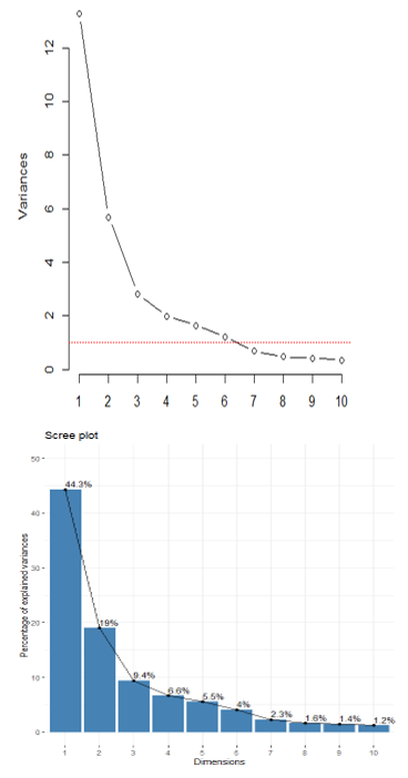
Fig 7: Scree plot for percentage of variances explained
The figure 7 shows the importance of the principal components and the variance explain where PC1 takes 44.3% of the total variance explained and the first five components take 85%. The first ten principal component explain the variance of 95%.
DISCUSSION
The procedure of examining and organizing the dataset for the diagnosis of breast cancer demonstrated a careful approach meant to guarantee the accuracy and applicability of the data for further stages of modeling. The work created a strong basis for insightful analysis by using popular datasets, like the Wisconsin Breast Cancer Database (WBCD), and adhering to accepted data science practices (Muhammet, 2020).
The original dataset, which included a number of attributes like radius, texture, perimeter, and more, was carefully preprocessed in the RStudio environment. This involved moving features around, eliminating columns that weren’t needed, such the ID, and making sure the diagnosis variable was properly labeled.Important insights into the features of the dataset were obtained through a thorough analysis of the data structure, normalization processes, and a balance check for the response variable (benign or malignant) (Akampurira Paul, 2022; Din, 2022).
One of the major issues that needed to be resolved during the data preparation stage was recognizing and managing multicollinearity. In order to guarantee the stability of the ensuing machine learning models, the study acknowledged the significance of looking at correlations between features. A thorough grasp of feature relationships was made easier by the use of Pearson correlation coefficients and visual aids such scatter diagrams and correlation plots (Brijith, 2023; Iqbal, 2022; Vogelstein, 2021).
Principal Component Analysis (PCA), one of the dimensionality reduction approaches introduced, showed how to strategically address the dataset’s high dimensionality (Kantardzic, 2020). The study effectively decreased the number of predictors while keeping a significant amount of the original variance by methodically converting the dataset into a lower-dimensional subspace. The screeplot and biplots gave useful information about the significance of the primary components and served as a guide for further modeling stages. (Chiu, 2015).
The outcomes discussion emphasizes how important these preliminary actions were in forming the latter stages of the investigation. In addition to addressing computing issues, the reduction in dimensionality improves the dataset’s interpretability, which is essential for efficient modeling (Kantardzic, 2020). PCA is a feature extraction method that has been chosen because it is appropriate for datasets that have correlated and redundant features, as determined by correlation checks (Jafari, 2024; Nwanganga, 2020).
The analysis of eigenvalues highlighted the significance of every principal component in adding to the variability of the dataset (Masters, 2020). A clear grasp of the declining returns in terms of variance explained by additional components was made possible by the visual representation of component importance using screeplots (Nwanganga, 2020).
CONCLUSION
The researcher was able to produce data from the data preparation and exploration phase that can be accessible from any data modeling program, such as IBM SPSS, Stata, Excel, R, etc. Effective data cleaning allowed us to generate clean data free of unsalvageable things. We generated subsets of the data that we used in the ensuing stages by reformatting and rescaling our features. Using correlational removal to eliminate strongly corelated characteristics, we were able to decrease our highly dimensional dataset of 30 predicting variables to 22 predicting variables. Additionally, we were able to maintain the accuracy of the predictive features while reducing the dimensionality of our data by at least 24% through the use of PCA for feature extraction.
ACKNOWLEDGEMENT
The completion of this work was made possible through the valuable contributions of several individuals. We extend our gratitude to the SOMAC and School of Science and Technology teams at Kampala International University for their dedicated efforts and support throughout the research process. Their expertise and commitment greatly enriched the quality of this project.
REFERENCES
- (IARC), I. A. (2018). Cancer burden rises to 18.1 million new cases and 9.6 million deaths in 2018. https://www.iarc.who.int/2018/09/pr263 E.
- 10.1259/bjr.20211033. Epub 2021 Dec 14. PMID: 34905391; PMCID: PMC8822551.
- Abuassba, A. O. M. (2017). Improving Classification Performance through an Advanced Ensemble Based Heterogeneous Extreme Learning Machines.
- AcadRadiol, G. M. (2002). Computer-aided diagnosis in radiology.
- AfefRania, L., et al. (2018). Comparison Study for Computer Assisted Detection and Diagnosis ‘CAD’ systems Dedicated to Prostate Cancer Detection Using MRImp Modalities.
- Ahmad, L. G., et al. (2015). Using three machine learning techniques for predicting.
- Akampurira Paul, S. P. (2022). Towards Ensemble Classification Algorithms for Breast Cancer Diagnosis in Women. DOI : 10.17577/IJERTV11IS060331.
- American Cancer Society. (2020). Cancer Facts and Figures, Atlanta, GA: American Cancer Society.
- American Cancer Society. (2020). Cancer Facts and Figures. Atlanta, GA: American Cancer Society.
- American Joint Committee on Cancer. (2017). Breast. In: AJCC Cancer Staging Manual. 8th ed. New York, NY: Springer.
- Arunachalam, A. (2017). Combining Heterogeneous Ensemble Learners Into a Single Meta-Learner in an Amateur Way.
- Asri, H. M. (2016). Using machine learning algorithms for breast cancer risk prediction and diagnosis.
- Ayer, T. (2011). Breast Cancer Risk Estimation with Artificial Neural Networks Revisited: Discrimination and Calibration.
- Balogh, E. P., et al. (2015). Improving Diagnosis in Health Care.
- Bashir, S. Q. (2015). Heterogeneous classifiers fusion for dynamic breast cancer diagnosis using weighted vote-based ensemble.
- Bekbolatova, M. M. (2024). Transformative Potential of AI in Healthcare: Definitions, Applications, and Navigating the Ethical Landscape and Public Perspectives. Healthcare, 12(2), 125. doi:10.3390/healthcare12020125.
- Black, E., et al. (2019). Improving early detection of breast cancer in sub-Saharan Africa: why mammography may not be the way forward.
- Bostock, M., et al. (2016). “Introducing Data Science: Big data, machine learning, and more, using Python tools.”
- Bowles, M. (2015). Machine Learning in Python Essential Techniques for Predictive Analysis.
- Bray F, L. M. (2022). Global cancer statistics 2022: GLOBOCAN estimates of incidence and mortality worldwide for 36 cancers in 185 countries. CA Cancer J Clin. 2024 Apr 4. doi: 10.3322/caac.21834. Epub ahead of print. PMID: 38572751.
- Bray F, Laversanne M, Sung H, Ferlay J, Siegel RL, Soerjomataram I, Jemal A. Global cancer statistics 2022: GLOBOCAN estimates of incidence and mortality worldwide for 36 cancers in 185 countries. CA Cancer J Clin. 2024 Apr 4. doi: 10.3322/caac.21834. Epub ahead of print. PMID: 38572751.
- Breit, C. A. (2019). Breast cancer risk assessment in patients who test negative for a hereditary cancer syndrome. The American Journal of Surgery.
- Brijith, A. (2023). Data Preprocessing for Machine Learning.
- Cao, B. Z. (2019). Classification of high dimensional biomedical data based on feature selection using redundant removal. DOI: 10.1371/journal.pone.0214406.
- Chan, Y.-T. (2020). An introduction to approaches and modern applications with ensemble learning.
- Chaurasia, V., et al. (2007). Data mining techniques: To predict and resolve breast cancer survivability.
- Chhatwal J, A. O. (2010). Optimal Breast Biopsy Decision-Making Based on Mammographic Features and Demographic Factors. Oper Res. 2010 Nov 1;58(6):1577-1591. doi: 10.1287/opre.1100.0877. PMID: 21415931; PMCID: PMC3057079.
- Chhatwal, J., et al. (2010). Optimal Breast Biopsy Decision-Making Based on Mammographic Features and Demographic Factors.
- Cortes, C., et al. (1995). Support-vector networks. Machine Learning.
- Das, S. a. (2019). Big data in healthcare: management, analysis and future prospects.
- Dhahri, H., et al. (2019). Automated Breast Cancer Diagnosis Based on Machine Learning Algorithms.
- Dietterich, T. G. (2020). Ensemble Methods in Machine Learning. Springer Berlin Heidelberg. Berlin, Heidelberg.
- Din, N. M. (2022). Breast cancer detection using deep learning: Datasets, methods, and challenges ahead. Computers in Biology and Medicine, 149, 106073.
- Elter, M. (2007). The prediction of breast cancer biopsy outcomes using two CAD approaches that both emphasize an intelligible decision process.
- F., N., et al. (2016). An automatic approach towards modal parameter estimation for high-rise buildings.
- Farrell S, M. A. (2022). Interpretable machine learning for high-dimensional trajectories of aging health. PLoS Comput Biol. 2022 Jan 10;18(1):e1009746. doi: 10.1371/journal.pcbi.1009746. PMID: 35007286; PMCID: PMC8782527.
- Faure, C. A. (2017). Empirical and fully Bayesian approaches for the identification of vibration sources from transverse displacement measurements. Mechanical Systems and Signal Processing.
- Forsyth, A., et al. (2018). Machine learning methods to extract documentation of breast cancer symptoms from electronic health records.
- Frankenfield, J. (2020). An introduction to Machine learning.
- Geneva: World Health Organization; 2024. Licence: CC BY-NC-SA 3.0 IGO.
- Habehh, H. &. (2021). Machine Learning in Healthcare. Current Genomics, 22(4), 291-300. https://doi.org/10.2174/1389202922666210705124359.
- Harris, J. R., et al. (2014). Physical Exam of the Breast. Diseases of the Breast. 5th ed. Wolters Kluwer Health.
- Hasan, H., et al. (2019). Feature selection of breast cancer based on principal component Analysis.
- Hazra, A., et al. (2016). “Study and Analysis of Breast Cancer Cell Detection using Naïve Bayes, SVM and Ensemble Algorithms.” International Journal of Computer Applications.
- Henry, N. L., et al. (2020). Cancer of the Breast. Here are the references in APA format:
- Hosni, M. H.-A.-A. (2019). Reviewing Ensemble Classification Methods in Breast Cancer.
- Huang J, C. P. (2021). Global incidence and mortality of breast cancer: a trend analysis. Aging (Albany NY).
- Huang J, Chan PS, Lok V, Chen X, Ding H, Jin Y, Yuan J, Lao XQ, Zheng ZJ, Wong MC. Global incidence and mortality of breast cancer: a trend analysis. Aging (Albany NY). 2021 Feb 11;13(4):5748-5803. doi: 10.18632/aging.202502. Epub 2021 Feb 11. PMID: 33592581; PMCID: PMC7950292.
- IARC. (2022). global cancer burden in 2022. https://gco.iarc.fr/today/fact-sheets-cancers.
- International Agency for Research on Cancer (IARC). (2018, September 12). Cancer burden rises to 18.1 million new cases and 9.6 million deaths in 2018. https://www.iarc.who.int/2018/09/pr263_E
- Iqbal, M. S. (2022). Breast Cancer Dataset, Classification and Detection Using Deep Learning. Healthcare, 10(12). https://doi.org/10.3390/healthcare10122395.
- Jafari, A. (2024). Machine-learning methods in detecting breast cancer and related therapeutic issues: a review. Computer Methods in Biomechanics and Biomedical Engineering: Imaging & Visualization, 1–11.
- Jemal, A., et al. (2011). Global cancer Statistics.
- Jia, W. S. (2022). Feature dimensionality reduction: a review. Complex Intell. Syst. 8, 2663–2693 (2022). https://doi.org/10.1007/s40747-021-00637-x.
- Jordan, M. I., et al. (2015). Machine learning: Trends, perspectives, and prospects.
- Kantardzic, M. (2020). Data Mining. Concepts, Models, Methods, and Algorithms 3ed.
- Katarzyna Kolasa, B. A.-V.-E. (2023). Systematic reviews of machine learning in healthcare: a literature review. https://doi.org/10.1080/14737167.2023.2279107.
- Khairunnahar, L. H. (2019). Classification of malignant and benign tissue with logistic regression.
- Li, W., et al. (2017). Extraction of modal parameters for identification of time-varying systems using data-driven stochastic subspace identification. Journal of Vibration and Control.
- Liew, X. Y., et al. (2021). A Review of Computer-Aided Expert Systems for Breast Cancer Diagnosis.
- Liu, N., et al. (2019). A novel intelligent classification model for breast cancer diagnosis.
- Madeh, P. S., & E., E.-D. T. (2020). Role of Data Analytics in Infrastructure Asset Management: Overcoming Data Size and Quality Problems.
- Maldonado, S. P. (2014). Feature selection for support vector machines via mixed integer linear programming.
- Masters, T. (2020). Modern Data Mining Algorithms in C++ and CUDA C: Recent Developments in Feature Extraction and Selection Algorithms for Data Science.
- Menagie, M. (2018). A comparison of machine learning.
- Muhammet, F. A. (2020). A Comparative Analysis of Breast Cancer Detection and Diagnosis Using Data Visualization and Machine Learning Applications. Healthcare (Basel).
- Mustafa, M., et al. (2016). Breast cancer: Detection markers, prognosis, and prevention. IOSR Journal of Dental and Medical sciences.
- Nematzadeh, Z., et al. (2015). Comparative studies on breast cancer classifications with k-fold cross validations using machine learning techniques.
- Noske, A. A. (2020). Risk stratification in luminal-type breast cancer: Comparison of Ki-67 with EndoPredict test results.
- Nwanganga, F., et al. (2020). Practical machine learning in R.
- Quinlan, J. (1996). Improved Use of Continuous Attributes in C4.5. Journal of Artificial Intelligence Research.
- Ricvan, D. N., et al. (2018). Diagnostic Accuracy of Different Machine Learning Algorithms for Breast Cancer Risk Calculation: a Meta-Analysis.
- Rokach, L. (2010). Ensemble-based classifiers.
- Salama, G. A. (2012). Breast cancer diagnosis on three different datasets using multi-classifiers.
- Setiono, R. (2000). Generating concise and accurate classification rules for breast cancer diagnosis. Artificial Intelligence Medicine.
- Shastry, K. S. (2022). Cancer diagnosis using artificial intelligence: a review. Artif Intell Rev 55, 2641–2673 (2022).
- Shen, R., et al. (2015). Intelligent breast cancer prediction model and clinical features: A comparative investigation in machine learning paradigm.
- Sidey-Gibbons, J. A. M., & Sidey-Gibbons, C. J. (2019). Machine learning in medicine: a practical introduction.
- Siegel, R. M. (2015). Cancer statistics, 2015. Ca A Cancer Journal for Clinicians.
- Singh, B. (2019). Determining relevant biomarkers for prediction of breast cancer using anthropometric.
- Thudumu, S. B. (2020). A comprehensive survey of anomaly detection techniques for high dimensional big data. J Big Data 7, 42 (2020). https://doi.org/10.1186/s40537-020-00320-x.
- Ting, F., et al. (2019). Convolutional neural network improvement for breast cancer classification. Expert Systems with Applications.
- Tobore, T. (2019). On the need for the development of a cancer early detection, diagnostic, prognosis, and treatment response system. Future Sci OA. 2019 Nov 29;6(2):FSO439. doi: 10.2144/fsoa-2019-0028. PMID: 32025328; PMCID: PMC6997916.
- Toğaçar, M., et al. (2020). Application of breast cancer diagnosis based on a combination of convolutional neural networks, ridge regression and linear discriminant analysis using invasive breast cancer images processed with autoencoders.
- Trieu, P. T. (2019). Improvement of cancer detection on mammograms via BREAST test sets.
- Uhlig, J., et al. (2019). Discriminating malignant and benign clinical T1 renal masses on computed tomography, A pragmatic radiomics and machine learning approach.
- Verboven, P. C. (2005). Improved total least squares estimators for modal analysis. Computer & Structure.
- Vogelstein, J. B. (2021). Supervised dimensionality reduction for big data. Nat Commun 12, 2872. https://doi.org/10.1038/s41467-021-23102-2.
- Vogelstein, J. T., et al. (2021). Supervised dimensionality reduction for big data. Nat Commun 12, 2872. https://doi.org/10.1038/s41467-021-23102-2
- Vrigazova, B., et al. (2019). Optimization of the ANOVA procedure for support vector machines. International Journal of Recent Technology and Engineering.
- Wang, H., et al. (2018). A support vector machine-based ensemble algorithm for breast cancer diagnosis.
- Wang, P., et al. (2020). Cross-task extreme learning machine for breast cancer image classification with deep convolutional features.
- Wang, S. W. (2019). An improved random forest based rule extraction method for breast cancer diagnosis.
- WHO global survey on the inclusion of cancer care in health-benefit packages, 2020–2021.
- WHO. (2021). global survey on the inclusion of cancer care in health-benefit packages. Geneva:: World Health Organization; 2024. Licence: CC BY-NC-SA 3.0 IGO.
- Wilkinson L, G. T. (2022). Understanding breast cancer as a global health concern. Br J Radiol. 2022 Feb 1;95(1130):20211033. doi:.
- Wilkinson L, Gathani T. Understanding breast cancer as a global health concern. Br J Radiol. 2022 Feb 1;95(1130):20211033. doi:
- Wilkinson, L., et al. (2021). Understanding breast cancer as a global health concern. https://doi.org/10.1259/bjr.20211033
- Witten, I. H., et al. (2011). Data Mining Practical Machine Learning Tools and Techniques.
- Wu, M., et al. (2019). Prediction of molecular subtypes of breast cancer using BI-RADS features based on a “white box” machine learning approach in a multi-modal imaging setting.
- Yaghoubi, V., et al. (2017). Automated Modal Parameter Estimation Using Correlation Analysis and Bootstrap Sampling. Mechanical Systems and Signal Processing.
- Yan, R., et al. (2019). Breast cancer histopathological image classification using a hybrid deep neural network.
- Zhang, X., et al. (2019). Extracting comprehensive clinical information for breast cancer using deep learning methods.
- Zonno, G., et al. (2017). Laboratory evaluation of a fully automatic modal identification algorithm using automatic hierarchical clustering approach. Procedia Engineering.
- Zumel, N., et al. (2020). Practical Data Science with R.