
Economic Policy Uncertainty and Financial Markets in the United State.
- Fadekemi Chidinma Adeloye
- Olayinka Olawoyin
- Chinaemerem Daniel
- 998-1016
- Jul 4, 2024
- Economics
Economic Policy Uncertainty and Financial Markets in the United State.
Fadekemi Chidinma Adeloye1*; Olayinka Olawoyin1; & Chinaemerem Daniel2
1Fox School of Business, Temple University, Philadelphia, USA
2Drexel University, Philadelphia, USA
*Corresponding Author
DOI: https://dx.doi.org/10.47772/IJRISS.2024.806076
Received: 15 May 2024; Revised: 01 June 2024; Accepted: 06 June 2024; Published: 04 July 2024
ABSTRACT
The economic space is ever-changing; hence, navigating the complexities of monetary policy uncertainty (EPU) and its ramifications on financial markets poses significant challenges for stakeholders. Policy uncertainty can lead to volatile market conditions, impacting investment decisions, capital flows, and overall economic stability. Thus, this study investigates this relationship by analyzing key variables such as stock market volatility, credit spreads, government bond yields, and trade volume. Utilizing secondary data from the Federal Revenue Economic (FRED) official website from 1990 to 2023, the study employs an autoregressive distributed lag model, incorporating an error correction mechanism and cointegration test. The findings indicate that stock market volatility (VI) has a significantly negative impact on market performance, demonstrating that increased volatility adversely affects market outcomes over extended periods. Moreover, the study observes relative stability in credit spreads, while trade volume and stock market volatility exhibit considerable fluctuations. While stock market volatility shows a significant negative impact on market performance, the effects of credit spreads and government bond yields are less evident. This study offers vital insights to policymakers, investors, and market participants, equipping them with knowledge to navigate uncertain financial environments and make informed decisions. Recommendations include strategies to mitigate the adverse effects of stock market volatility and foster stability in financial markets for sustainable economic growth.
Keywords: Economic Policy Uncertainty, financial markets, stock market volatility, credit spreads, government bond yields, trade volume, and economic stability
INTRODUCTION.
Economic policy uncertainty (EPU) significantly impacts investors, financial institutions, economists, analysts, and policymakers, particularly within the financial market. This uncertainty influences investment decisions, market behavior, and overall economic performance, especially during political and civil unrest. Policymakers and financial analysts use market fluctuations to forecast company health and investment outlooks, identifying stock market risks for informed decision-making. Understanding the relationship between financial markets and EPU is crucial for ensuring financial stability through research, risk management, and portfolio selection. Studies have shown that financial markets fluctuate following political shocks (Sahinoz & Erdogan, 2018; Bakhsh & Zhang, 2023).
In recent decades, several events have increased uncertainty surrounding US economic policy. The 2008 global financial crisis led to a slow recovery, with the highest unemployment rate in post-war history at 7.8% (Hardouvelis et al., 2018). The 2018 economic conflict between China and the US further exacerbated this uncertainty, with tariffs impacting significant portions of both economies’ GDPs (Fajgelbaum et al., 2023). The COVID-19 pandemic added to this uncertainty, increasing the EPU index significantly during polarized presidential elections. As of March 2024, the US EPU index reached a record high of 94.12 (Trading Economics, 2024). To address this uncertainty, Baker et al. (2016) developed the EPU index, derived from ten widely read US newspapers. This study incorporates three new EPU indices by Baker, Davis, and Levy (2022), focusing on policy uncertainty from state, local, national, and international sources. This data, collected monthly, will be converted to annual data using averaging methods for analysis.
This study will analyze the EPU Index and the financial market using descriptive statistics on stock market trading, investment, and GDP. It will compare the financial market’s performance before and after significant events like the Great Recession, the COVID-19 pandemic, and political elections. Given the ongoing US-China trade war, a univariate or bivariate predictive regression model will be used to forecast the financial market. The study will also compare the EPU index’s performance with other macroeconomic factors and EPU indices, assessing its ability to forecast stock prices, market value, investment, and overall economic performance. Empirical studies suggest EPU affects financial markets by delaying financial decisions, reducing consumption and investments, increasing unemployment, and raising capital expenses.
To evaluate the predictive performance of the EPU index, R-squared (R²) statistics will be used with out-of-sample data to assess its generalizability. Most empirical studies find higher EPU levels negatively impact organizational performance, while positive adjustments promote growth. Some studies, such as those by Liu et al. (2023) and Sharif et al. (2020), use wavelet-based approaches to examine EPU’s effects. However, the use of the EPU index to predict financial markets during periods of unrest or shock has received limited attention. Given the recent increase in the US EPU index, examining its impact on the financial market is crucial, focusing on stock prices, investment, market behavior, and economic performance.
LITERATURE REVIEW
2.1 Conceptual Review
Economic Policy Uncertainty (EPU) represents a multifaceted construct encompassing the unpredictability surrounding economic policies, including fiscal, monetary, and regulatory measures (Dakhlaoui & Aloui, 2016; Adjei & Adjei, 2017). It reflects the dynamic and fluctuating nature of policy decisions, leading to ambiguity and hesitation among investors, businesses, and policymakers. The significance of EPU lies in its ability to disrupt economic decision-making processes and influence market sentiments (Baker, Bloom, & Davis, 2016).
Stock market volatility, often a key barometer of market uncertainty and risk, reflects the degree of fluctuation or change in stock prices over a specified period (DLM – a Development Investment Bank, 2024). This phenomenon holds significant implications for investors, influencing their investment decisions, portfolio management strategies, and overall market sentiment. Investors encounter various types of risks within the realm of stock market volatility, categorized into systematic and unsystematic risks (Li et al., 2022). Systematic risks, such as economic factors, geopolitical events, and market sentiment, impact the broader market or specific segments, while unsystematic risks are specific to individual assets or companies, influenced by factors like company performance and regulatory changes. Economic indicators, corporate news, geopolitical events, and investor sentiment serve as primary drivers of stock market volatility (Goonatilake & Herath, 2007), shaping market behaviors and investment outcomes.
Credit spreads are essential indicators for credit investors, guiding their understanding of the compensation received for bearing credit risk within a security (O’Kane & Sen, 2005). Whether embedded within corporate or sovereign bonds or synthesized through credit derivatives, credit risk can vary across securities due to differences in maturity, coupon, or seniority. These spreads facilitate comparisons within a company’s bond offerings and across different issuers, assisting investors in identifying relative value opportunities (O’Kane & Sen, 2005). Credit spreads enable comparisons across various credit instruments, including fixed-rate bonds, floating-rate bonds, asset swaps, and default swaps, allowing investors to assess pricing fairness relative to benchmark rates such as the government curve or Libor swap rate (O’Kane & Sen, 2005). Despite multiple measures of credit spreads, they all fundamentally represent the yield differential between two debt instruments with the same maturity but differing credit ratings (Loo, 2023). These spreads encompass compensation for anticipated default losses alongside a risk premium, underscoring the intricate relationship between credit quality and investment returns (Kaviani et al., 2020).
2.2 Empirical Review
Empirical studies comprehensively review the relationship between economic policy uncertainty (EPU) and the financial market. Numerous scholars have contributed to understanding the impact of EPU on stock market volatility and trading behavior across different countries and regions. Smales (2020) investigated the relationship between policy and financial market uncertainty across the G7 economies. Using the EPU measure developed by Baker et al. (2016), the study found that financial market uncertainty, measured by implied volatility, increases as economic policy uncertainty rises, particularly during periods of economic weakness. The study controlled for macroeconomic state variables and country/time fixed effects, demonstrating that US and Japanese policy uncertainty significantly affect global financial market uncertainty, indicating a spill-over effect consistent with the size of their economies.
Ghani and Ghani (2023) focused on Pakistan’s stock market volatility and examined the impact of EPU indices from Pakistan and its global trading partners, including the US, China, and the UK. Employing the GARCH-MIDAS model and combination forecast approach, the study found that the US economic policy uncertainty index is a powerful predictor of Pakistan’s stock market volatility. Surprisingly, Pakistan and China’s EPU indices do not provide significant predictive information during the sample period, while the UK’s EPU index also influences equity market volatility prediction.
Javaheri, Habibi, and Amani (2022) investigated the impact of economic policy uncertainty and economic factors on the US stock market index using Non-ARDL and Quantile models. The study found that declining economic and economic-political factors increase the US stock market index. Also, the effect of inflation and GDP variables follows a nonlinear pattern, revealing asymmetric impacts on stock market transactions. Khojah et al. (2023) examined the asymmetric effect of economic policy uncertainty on stock prices in G7 countries using a panel threshold approach. Contrary to previous research, the study uncovers evidence of an asymmetric effect, where increased policy uncertainty initially positively impacts stock prices up to a certain threshold, beyond which it turns negative. These findings align with various hypotheses in finance, including information asymmetry, prospect theory, behavioral finance, and market liquidity, highlighting the nuanced behavior of stock prices in response to changing levels of policy uncertainty.
Adam, Sidek, and Sharif (2022) examined the impact of global economic policy uncertainty and volatility on stock markets in Islamic countries. Utilizing wavelet coherence ratios, the study reveals that economic policy uncertainty generally exerts a negative effect on Islamic stock returns, except the Dow Jones Islamic Market (DJIM). Conversely, volatility notably positively impacts most Islamic stock returns, particularly following the COVID-19 outbreak. Furthermore, Albrecht, Kapounek, and Kučerová (2023) investigated the co-movements between EPU and selected stock market indices (S&P500, UK100, Nikkei225, and DAX30) at different investment horizons. They found that EPU lags stock markets at longer investment horizons, especially during global financial turmoil, with identified lag ranging between 2 and 6 months for investment horizons exceeding 32 months. They also found that short-term effects of EPU on stock markets are confirmed.
Škrinjarić and Orlović (2020) focused on the spillover effects of EPU shocks on stock market returns and risks for selected Central and Eastern European (CEE) markets. Using vector autoregression (VAR) models and Spillover Indices, their study provides insights into the sources of shock spillovers between EPU and stock market variables, offering recommendations for policymakers and international investors. Olanipekun, Olasehinde-Williams, and Güngör (2019) examined the impact of EPU on exchange market pressure, capturing changes in foreign reserves and exchange rates. They found a long-run relationship between exchange market pressure and EPU, with a rise in EPU increasing the severity of exchange market pressure. The study highlights the role of various domestic and external factors in mitigating the effect of exchange market pressure.
In India, Mishra et al. (2023) investigated the impact of directional global EPU on the Indian stock market volatility using the GARCH-MIDAS approach. They disintegrated global EPU into its components and tested their linkages with Indian stock market volatility, finding a positive and significant impact of global EPU on Indian capital market volatility. The study also examines the dynamic directions of EPU and its predictive power for Indian stock market uncertainty. In Europe, particularly in Canada, Batabyal and Killins (2021) made a notable contribution to the literature by examining the impact of economic policy uncertainty (EPU) on Canadian stock market returns spanning from 1985 to 2015. Their study found significant negative impacts of EPU on Canadian stock market returns in both OLS and ARDL estimations, with asymmetric effects observed in the short and long run. Aydin, Pata, and Inal (2022) investigated the causal relationship between EPU and stock prices in BRIC countries using asymmetric and symmetric frequency domain causality tests. They found unidirectional permanent causality from EPU to stock prices for Brazil and India, bidirectional causality for China, and differential effects of positive and negative components of EPU on stock prices. All of these studies across regions collectively contribute to the understanding of the impact of EPU on financial markets, providing valuable insights for policymakers, investors, and researchers.
2.3 Theoretical Framework
The study’s theoretical framework draws upon the Efficient Market Hypothesis (EMH) and Behavioral Finance Theory to elucidate the relationship between economic policy uncertainty and financial market dynamics. The Efficient Market Hypothesis (EMH) posits that financial markets promptly incorporate all available information into asset prices, making it difficult for investors to outperform the market without assuming greater risk (Vamvakaris et al., 2017; Lucas Downey, 2024). Developed by Samuelson and Fama, EMH suggests that assets in efficient markets consistently trade at their intrinsic value, rendering attempts to identify undervalued stocks or forecast market trends through analysis futile (Lucas Downey, 2024). EMH contends that neither technical nor fundamental analysis reliably generates risk-adjusted excess returns, except through insider information (Lucas Downey, 2024). The theory suggests that investors benefit most from adopting passive strategies, focusing on low-cost, diversified portfolios rather than active trading or market timing. EMH posits that stock analysis and timing strategies provide no added value, as potential opportunities for excess returns are quickly seized and nullified by other market participants in efficient markets (Vamvakaris et al., 2017). Despite its importance in financial theory, EMH remains contentious. Critics argue that market anomalies and behavioral biases challenge EMH’s assumptions, proposing that certain investors may consistently outperform the market using superior information or analytical techniques (Vamvakaris et al., 2017). Moreover, empirical evidence of market inefficiencies and anomalies casts doubt on the concept of perfect market efficiency posited by EMH. Nonetheless, EMH continues to influence investment strategies, regulatory frameworks, and academic research in financial economics.
Behavioral Finance Theory offers insights into why individuals often make irrational financial decisions driven by emotions rather than rationality (William & Mary, 2024; Rajesh Kumar, 2016; Prosad et al., 2015). Rooted in the idea that investors are not always rational actors, behavioral finance utilizes principles from financial psychology to scrutinize investors’ actions, revealing cognitive biases and limited self-control that led to judgment errors (William & Mary, 2024). The theory traces its roots back to George Seldon’s “Psychology of the Stock Market” in 1912 but gained significant momentum in 1979 with the groundbreaking work of Daniel Kahneman and Amos Tversky (William & Mary, 2024). Their research laid the foundation for understanding how subjective reference points influence decision-making, challenging the assumptions of traditional economic theories (William & Mary, 2024). Subsequently, Richard Thaler introduced the concept of mental accounting, highlighting how individuals perceive money differently based on its designated purpose (William & Mary, 2024). These pioneering contributions set the stage for studying cognitive biases and behavioral anomalies in finance. Behavioral finance provides explanations for market inefficiencies by delving into the psychological influences on financial practitioners’ behavior (Rajesh Kumar, 2016). Kahneman and Tversky’s prospect theory, for instance, underscores how individuals’ overweight recent experiences and exhibit overconfidence in their beliefs, leading to distorted risk perceptions. Other biases, such as conservatism bias and regret avoidance, further shape decision-making processes, affecting market dynamics and asset prices. In practice, behavioral biases often manifest in investors’ tendencies to follow trends or patterns in market prices, as observed in technical analysis. Technical analysts leverage behavioral biases to identify trends and patterns, contributing to the persistence of certain market phenomena. However, such biases challenge the efficient market hypothesis, suggesting that market prices may deviate from their intrinsic values due to psychological factors (Prosad et al., 2015).
MATERIALS AND METHOD
The research design adopted for this study is an ex-post facto approach, facilitating the exploration of relationships between variables that have already occurred without direct manipulation by the researcher, which is well-suited for investigating the nexus between Economic Policy Uncertainty (EPU) and financial market variables. EPU is assessed using three key indicators: Stock Market Volatility, Credit Spreads, and Government Bond Yields, with Stock Market Volatility measuring the degree of fluctuation in stock prices, Credit Spreads quantifying the difference in yields between different debt instruments with the same maturity but different credit ratings, and Government Bond Yields indicating the returns on bonds issued by governments, reflecting economic policy uncertainty. Trading volume will be utilized as a proxy for the dependent variable, representing the financial market. This measure captures the level of activity and liquidity in the financial market.
Government bond yield plays a key role in financial markets, serving as a vital indicator of economic conditions, monetary policy expectations, and investor sentiment. The concept of government bonds revolves around borrowing mechanisms employed by sovereign entities to finance various initiatives, including infrastructure projects and public spending. Further explained by the Reserve Bank of Australia (2024), the yield curve derived from government bonds helps to understand the interest rate expectations and their transmission mechanisms throughout the economy. This yield curve reflects a series of bond yields across different maturities, providing crucial information for investors, policymakers, and market analysts. Government bonds are widely regarded as safe investments due to the backing of sovereign entities, granting them control over currency issuance and reducing default risk. However, factors such as political stability, macroeconomic conditions, and creditworthiness contribute to variations in bond yields across different countries, as highlighted by Brooks Macdonald (2024). Bond yields demonstrate an inverse relationship with bond prices, as Hayes (2024) outlined, wherein rising interest rates result in lower bond prices and vice versa. Understanding bond yields is crucial for investors as it allows them to evaluate investment returns, manage portfolio risk, and navigate market fluctuations effectively. Government bond yields, in particular, serve as critical benchmarks in financial markets, influencing a wide range of interest rates and economic activities.
Financial markets serve as vital channels for trading various financial instruments, including bonds, equities, currencies, and derivatives, enabling the exchange of capital between investors and borrowers (Financial Markets, 2024; Mishura, 2016). These markets play a crucial role in capitalist economies by allocating resources efficiently and providing liquidity for businesses and entrepreneurs (Mishura, 2016). Despite their diversity, financial markets can generally be categorized into segments such as the stock market, bond market, forex market, and derivatives market (OCC, 2024). Each of these markets serves distinct functions within the broader financial ecosystem, catering to the diverse needs of market participants. However, financial markets are subject to various external influences, including economic conditions, geopolitical events, and the actions of market participants, leading to random fluctuations in asset prices over time (Mishura, 2016).
Trade volume is a fundamental aspect of financial markets and represents the total quantity of shares or contracts exchanged for a specific security within a defined time period (Twin, 2024). It serves as a critical measure of market activity and liquidity, reflecting the level of engagement between buyers and sellers during trading hours. High trade volumes are generally viewed positively as they indicate greater liquidity and improved order execution, whereas low trade volumes may suggest reduced market activity and liquidity. The concept of trade volume is intertwined with the dynamics of stock markets, where both volume and prices are influenced by underlying economic forces, providing valuable insights into market functioning (Lo & Wang, 2010). In equilibrium, the interaction between prices and volumes carries significant implications for asset pricing models. This interaction enables the identification of hedging portfolios that can be utilized to hedge against changes in market conditions.
3.1 Data sources
The data for this study will be sourced from the Federal Reserve Economic Data (FRED) official website. Specifically, the dataset will include relevant variables crucial for evaluating the impact of Economic Policy Uncertainty (EPU) on financial market variables. The key variables of interest are Stock Market Volatility, Credit Spreads, Government Bond Yields, and trading volume covering the period from 1990 to 2023. These variables will be instrumental in analyzing the relationships between EPU and financial market dynamics
3.2 Measurement of Variable
| S/N | Variable Name | Definition | Supporting Literature | Source of Data |
| 1 | Economic Policy Uncertainty | Independent Variable | ||
| Stock Market Volatility (VI) | The degree of fluctuation in stock prices over a specific period, reflecting market uncertainty and risk. | Ozili (2021);
Ghani and Ghani, (2023); Adam, Sidek, and Sharif, (2022). |
Chicago Board Option Exchange | |
| Credit Spreads (CS) | The difference in yields between debt instruments of the same maturity but with varying credit ratings. | Ozili (2021);
Ghani and Ghani, (2023); Adam, Sidek, and Sharif, (2022). |
Organization for economic corporation and development (OECD) | |
| Government Bond Yields (GBY) | The returns on bonds issued by governments, reflecting economic policy uncertainty. | Ozili (2021);
Ghani and Ghani, (2023); Adam, Sidek, and Sharif, (2022). |
Organization for economic corporation and development (OECD) | |
| 2 | Financial market | Dependent Variable | ||
| Trade volume (TV) | The total volume of trading activity in a financial market within a specific period. | Ozili (2021);
Ghani and Ghani, (2023); Adam, Sidek, and Sharif, (2022). |
Organization for economic corporation and development (OECD) |
3.3 Model Estimation
The autoregressive distributed lag (ARDL) model is used in econometrics to analyze the relationship between variables over time. The model specification involves determining the order of the autoregressive and distributed lag terms and selecting the appropriate variables to include in the model.
\[
\Delta Y_t = \alpha + \beta_1 \Delta Y_{t-1} + \beta_2 \Delta Y_{t-2} + \ldots + \beta_p \Delta Y_{t-p} + \gamma_0 \Delta X_{t-1} + \gamma_1 \Delta X_{t-2} + \ldots + \gamma_q \Delta X_{t-q} + \epsilon_t…………………………………………………general ARDL
\]
\[
\Delta Y_t = \alpha + \beta_1 \Delta Y_{t-1} + \beta_2 \Delta Y_{t-2} + \beta_3 \Delta Y_{t-3} + \gamma_0 \Delta X_{t-1} + \gamma_1 \Delta X_{t-2} + \gamma_2 \Delta X_{t-3} + \epsilon_t………………………………………main model
\]
Where:
- Yt presents the dependent variable at time t;
- Yt-1,. . . ,Yt-p are the lagged values of the dependent variable;
- Xt-1,. . . ,Xt-q are the lagged values of the independent variables;
- α is the intercept or constant term;
- β1,…,βp are the coefficients of the lagged differences of Yt
- γ0,γ1,… ,γq are the coefficients of the lagged differences of Xt
- ϵt represents the error term at time t.
3.4. Method of Data Analysis
To investigate the relationships between Economic Policy Uncertainty (EPU) and financial market variables in the United States, we will employ an autoregressive distributed lag (ARDL) modeling approach. This econometric technique is well-suited for analyzing dynamic relationships over time, particularly in assessing the impact of EPU on financial market behavior. The ARDL model will determine lag orders for the dependent (financial market variables) and the independent (EPU) variables, incorporating lagged effects to account for time dynamics. The dependent variables (financial market) will be measured using Trading Volume. At the same time, EPU will serve as the key independent variable and use proxies such as Stock Market Volatility, Credit Spreads, and Government Bond Yields. Equations within the ARDL model will assess the significance of relationships and provide insights into the short- and long-term effects of EPU on financial market variables. Estimation will be conducted using statistical software such as EViews or STATA, with diagnostic tests ensuring the robustness of the model. Results will offer valuable insights into the magnitude and direction of the relationship between EPU and financial market variables, thereby informing stakeholders and policymakers about the implications for investment decisions and economic stability in the United States.
DATA ANALYSIS
4.1 Descriptive Analysis
The descriptive analysis provides valuable insights into various aspects of the US financial markets from 1990 to 2023. Credit Spread (CS), representing the difference in yield between corporate and government bonds, shows an average spread of 0.64%. With a low standard deviation of 0.53, credit spreads appear relatively stable, though the range from -0.52 to 4.08 indicates some variability, potentially influenced by market conditions over the period. Moreover, the positive skewness of 1.31 suggests a slightly right-skewed distribution, while a kurtosis of 6.69 indicates heavier tails and a sharper peak, highlighting potential extreme values or volatility spikes.
Government Bond Yield (GBY), reflecting the returns on government bonds, exhibits an average yield of 4.25%, with a moderate standard deviation of 1.99. The range from 0.62 to 8.89 illustrates the variability in bond yields, potentially influenced by economic factors and market conditions. Despite a skewness close to 0.31, indicating near symmetry in the distribution, a negative kurtosis of -0.8 suggests relatively moderate risk or volatility associated with government bond yields compared to CS.
Trade Volume (TV), representing market activity, shows an average volume of 1.82, with a high standard deviation of 4.22, indicating considerable variability around the mean. The wide range from -15.76 to 40.76 reflects substantial fluctuations in market activity, potentially influenced by trading patterns, economic events, and investor sentiment. A positive skewness of 1.54 indicates a right-skewed distribution, with occasional high-volume trading days. At the same time, a kurtosis of 20.84 suggests heavy tails and a sharp peak, indicating potential extreme values or volatility spikes.
Stock Market Volatility (VI), representing market risk, exhibits an average volatility of 19.59, with a high standard deviation of 7.55, suggesting significant variability in market volatility over the observed period. The range from 10.13 to 62.67 reflects substantial fluctuations in market conditions and investor uncertainty. Furthermore, a positive skewness of 1.98 suggests occasional spikes in volatility. At the same time, a kurtosis of 6.59 indicates heavier tails and a sharper peak, indicating potential extreme values or volatility spikes in stock market volatility. These descriptive statistics offer valuable insights into the dynamics and characteristics of the US financial markets during the specified timeframe.
Table 1: Summary Statistics of the variables
| Mean | SD | Minimum | Maximum | Range | Skewness | Kurtosis | |
| CS | 0.64 | 0.53 | -0.52 | 4.08 | 4.6 | 1.31 | 6.69 |
| GBY | 4.25 | 1.99 | 0.62 | 8.89 | 8.27 | 0.31 | -0.8 |
| TV | 1.82 | 4.22 | -15.76 | 40.76 | 56.52 | 1.54 | 20.84 |
| VI | 19.59 | 7.55 | 10.13 | 62.67 | 52.54 | 1.98 | 6.59 |
4.2 Trend Analysis
A. Trend Analysis of Credit Spread
The trend analysis for credit scores reveals a uniform pattern beginning from 1990 and experiencing a surge increase around 2010 with a decrease and continuing to progress uniformly thereafter. This implies there existed a sudden increase in credit scores around 2010.
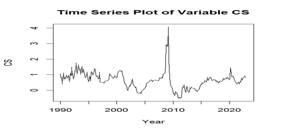
Figure 1. Time Series Plot of Credit Score.
B. Trend Analysis of Government Bond Yield
Fig. 2 shows the trend analysis for Government Bond Yield, which reveals a negative decline from 1990. There is a small increase starting in the year 2020, but there was a sudden rise in credit scores around 2010.
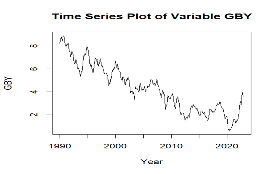
Figure 2. Time Series Plot of Government Bond Yield
C. Trend Analysis of Financial Market (Trade Volume)
The trend analysis of Trade Volume shown in Fig. 4.3 initially displays a uniform pattern from 1990, followed by a negative decrease around 2010, before experiencing a uniform positive increase. However, a sharp negative decrease and a strong positive increase were observed around 2020.
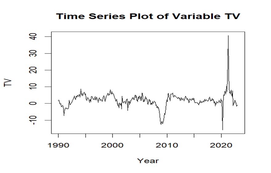
Figure 3. Time Series Plot of Trading Volume.
D. Trend Analysis of Stock Market Volatility
Fig. 4. shows the trend analysis for stock Market Volatility, which first reveals there appears to be an uniform decrease from 1990, a noticeable increase in 2000, back to a negative decline and a surge increase in 2010. Then there is a uniform a uniform pattern from 1990 and a negative decrease around 2010 before a uniform positive increase. However, a sharp negative decrease and a strong positive increase were observed around 2020.
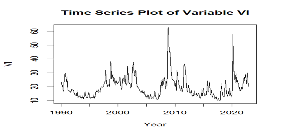
Figure 4. Time Series Plot of Market Volatility
4.3 Stationarity Test
The stationary test results provide insights into the stationarity of the variables analyzed, namely Credit Spread (CS), Government Bond Yield (GBY), Trade Volume (TV), and Stock Market Volatility (VI). Stationarity is an important concept in time series analysis, it indicates whether the statistical properties of a series remain constant over time. For Credit Spread (CS), the Augmented Dickey-Fuller (ADF) test yields a test statistic of -4.007 for the case of no lag (l(0)) and -7.688 for one lag (l(1)). Both test statistics are highly significant at the 1% level (***), indicating strong evidence against the presence of a unit root in the series. Consequently, CS can be considered stationary, implying that its mean, variance, and autocovariance are constant over time. Similarly, Government Bond Yield (GBY) exhibits significant results with test statistics of -3.274 for no lag and -7.167 for one lag, both significant at the 1% level (***). This suggests that GBY is also stationary, indicating a stable behavior in bond yields over the analyzed period. Trade Volume (TV) displays significant results with test statistics of -3.86 for no lag and -8.26 for one lag, important at the 5% level (**). These results imply that TV is stationary, suggesting consistent trading activity in the financial markets without systematic shifts in volume over time.
Lastly, Stock Market Volatility (VI) demonstrates significant results with test statistics of -3.78 for no lag and -9.475 for one lag, important at the 5% and 1% levels (** and ***), respectively. These findings indicate that VI is stationary, implying that the level of volatility in the stock market remains relatively constant over the specified period.
Table 2. ADF for Stationarity Test
| Variable | ADF(l(0)) | ADF(l(1)) |
| CS | -4.007*** | −7.688*** |
| GBY | −3.274 | −7.167*** |
| TV | −3.86** | −8.26*** |
| VI | -3.78** | -9.475*** |
* Significance at 10%, ** Significance at 5%, *** Significance at 1%. The asterisks indicate the rejection of the null hypothesis of unit root.
4.4 Cointegration Test
The cointegration test results provide insights into the long-term relationships between the variables included in the model: Financial Market GDP (FGDP), Trade Volume (TV), Credit Spread (CS), Government Bond Yield (GBY), and Stock Market Volatility (VI). Cointegration is a crucial concept in time series analysis, indicating whether the variables move together in the long run despite short-term fluctuations. In this analysis, the model tested is FGDP (TV|VI, CS, GBY), suggesting that Financial Market GDP depends on Trade Volume, Stock Market Volatility, Credit Spread, and Government Bond Yield. The cointegration test yields an F-statistic of 4.03, which is highly significant at the 1% level (***). This result indicates strong evidence of cointegration among the variables included in the mode.
The interpretation of cointegration in this context suggests a long-term relationship exists among FGDP, TV, CS, and GBY, with VI potentially influencing this relationship. This implies that while individual variables may exhibit short-term fluctuations, they move together in the long run due to their interconnectedness or shared underlying factors.
Overall, the cointegration test results suggest that FGDP, TV, CS, and GBY are cointegrated, indicating a stable and long-term relationship among these variables in the context of the analyzed financial markets. This finding has important implications for understanding the dynamics and interdependencies within the economic system and can inform more robust modeling and forecasting efforts.
Table 3. Results of Cointegration test.
| Model | F-Statistic | Result | |
| FGD (TV|VI, CS, GBY) | ARDL (1, 1, 1) | 4.03*** | Cointegration |
4.5 Long-Run and Error Correction Model
The long-term analysis provides crucial information on the relationship between dependent and independent variables over an extended period. The constant term in the table represents the exact dependent variable. The constant term (C) of 0.005 suggests a baseline level of the dependent variable, potentially close to zero. However, the confidence interval [-0.042] indicates some uncertainty in this estimate, highlighting the need for caution in interpreting this coefficient. Stock Market Volatility (VI) emerges as a significant predictor in the long run, with a coefficient of -0.11***. This implies that the dependent variable decreases by 0.11 units on average for each unit increase in Stock Market Volatility. The significance level (***), along with the t-statistic value of -3.263, provides strong evidence of the negative impact of VI on the dependent variable.
On the other hand, the coefficients for Credit Spread (CS) and Government Bond Yield (GBY) don’t seem to be statistically significant predictors of the dependent variable over the long term Although CS has a coefficient of -0.51, suggesting a potential negative impact on the dependent variable, the confidence interval [-0.726] includes zero, indicating uncertainty in this estimate. Similarly, GBY’s coefficient of 0.17, which implies a positive impact, has a confidence interval [0.269] that encompasses zero, suggesting ambiguity in the relationship.
In summary, Stock Market Volatility (VI) demonstrates a significant negative impact on the dependent variable in the long run. However, the effects of Credit Spread (CS) and Government Bond Yield (GBY) are not as evident. Further analysis and consideration of potential factors influencing these relationships may be necessary to improve comprehension and guide decision-making in the analyzed financial markets.
Table 4. Long-run Coefficients.
| Variables | Coefficient | t-statistic | P-value |
| Constant | 0.005 | -0.042 | 0.001*** |
| VI | -0.11 | -3.263 | 0.000*** |
| CS | -0.51 | -0.726 | 0.103 |
| GBY | 0.17 | 0.269 | 0.211 |
Where *** indicates p-value < 0.05 (5% significance level)
4.6 Error Correction Model
The error correction analysis provides valuable insights into the immediate effects of Stock Market Volatility (VI), Credit Spread (CS), and Government Bond Yield (GBY) on the dependent variable, likely Financial Market GDP (FGDP) or another relevant economic indicator. Each coefficient in the error correction estimates indicates the effect of a one-unit increase in the corresponding independent variable on the dependent variable. Stock Market Volatility (VI) demonstrates statistically significant positive effects on the dependent variable, with a coefficient of 0.0598*. This suggests that for every unit increase in VI, the dependent variable increases by an average of 0.0598 units. This relationship is significant at the 10% level, indicating an immediate influence of stock market volatility on the dependent variable. Credit Spread (CS) demonstrates a highly significant positive impact on the dependent variable, with a coefficient of 1.3247***. This implies that for each unit increase in CS, the dependent variable increases by 1.3247 units on average in the error correction. The significance level of *** highlights the solid statistical evidence supporting the immediate effect of credit spread on the dependent variable.
Government Bond Yield (GBY) significantly affects the dependent variable, with a coefficient of 1.5134**. This suggests that for each unit increase in GBY, the dependent variable increases by 1.5134 units on average in the error correction. The significance level of ** underscores the statistical significance of the relationship between government bond yields and the dependent variable. Moreover, the high Adjusted R-squared (Adj. R2) value of 0.84 indicates that VI, CS, and GBY collectively explain 84% of the variation in the dependent variable in the error correction. This highlights the solid explanatory power of the model for capturing short-term fluctuations in the dependent variable. Additionally, the presence of positive autocorrelation in the model residuals is indicated by the Durbin-Watson statistic (D-W stat) of 2.17* at the 10% significance level. This suggests a potential serial correlation in the errors, requiring further investigation to ensure the robustness of the model. Furthermore, the absence of heteroskedasticity in the model residuals is supported by the ARCH test (Het) results, with a value of 2.403 and a p-value of 0.4931. This indicates that the variance of the errors remains constant over time, enhancing the reliability of the model estimates. Overall, the error correction analysis highlights the immediate impacts of Stock Market Volatility (VI), Credit Spread (CS), and Government Bond Yield (GBY) on the dependent variable, with significant statistical evidence and a strong explanatory power of the model. However, positive autocorrelation in the model residuals warrants attention, while the absence of heteroskedasticity enhances the reliability of the model estimates.
Table 5. Error Correction Model
| Variables | Coefficients | P-value |
| Constant | 0.061 | 0.000*** |
| VI | 0.0598 | 0.071* |
| CS | 1.3247 | 0.000*** |
| GBY | 1.5134 | 0.031** |
| Adj. R2 | 0.84 | |
| D-W stat | 2.17* (0.06) | |
| Het | 2.403 (0.4931) |
Where:
*: Significant at the 10% level
**: Significant at the 5% level
***: Significant at the 1% level
Notes: Adj. R2 means Adjusted R-squared. Het is the ARCH test for t-statistics in [], and p-values in ().
4.7 Diagnostic and Stability Tests
According to the diagnostic tests in Table 3, none of the specified Autoregressive Distributed Lag (ARDL-Bounds) models show heteroscedasticity. The coefficients of the ARDL model remain stable across all specifications, as illustrated by Figures 1 and 2. These figures indicate that the cumulative sum of recursive residuals (CUSUM) falls within the critical bounds for the 5% significance level.
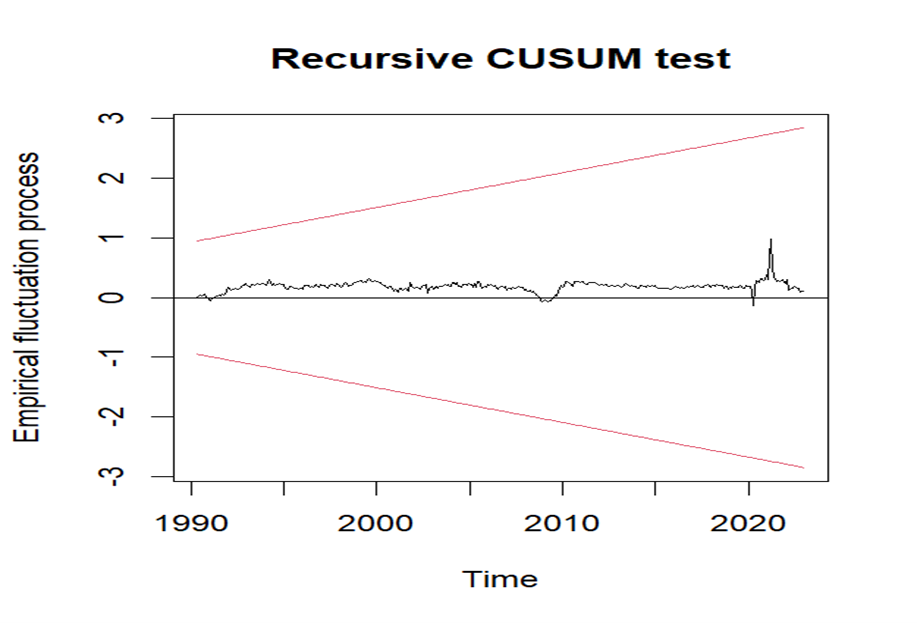
Figure 5. Plot of CUSUM for coefficient stability of Error Correction term (ECM) model 1
4.5 Discussion of Findings
The descriptive analysis reveals the characteristics of the financial market variables under study. Credit spread (CS) demonstrates relative stability with a low standard deviation, which means it is consistent over time. This discovery is consistent with prior research, which suggests that credit spread remains stable as a marker of market sentiment and risk perception (Albrecht et al., 2023). However, the moderate variability in government bond yield (GBY) and considerable fluctuations in trade volume (TV) and stock market volatility (VI) highlight the dynamic nature of financial markets, influenced by various economic factors and investor sentiment (Batabyal & Killins, 2021; Škrinjarić & Orlović, 2020).
Trend analysis reveals distinct patterns in the behavior of financial market variables over time. The surge increase in credit spread (CS) around 2010 corresponds to periods of economic uncertainty and financial distress, impacting investor risk perception (Albrecht et al., 2023). Similarly, the negative decline in government bond yield (GBY) and fluctuations in trade volume (TV) and stock market volatility (VI) reflect changing market dynamics influenced by economic events and policy decisions (Mishra et al., 2023). The stationarity test confirms the stability of credit spread (CS), government bond yield (GBY), trade volume (TV), and stock market volatility (VI) over time. This finding is consistent with the notion that these variables exhibit consistent statistical properties, allowing for reliable analysis and modeling of financial market behavior (Olanipekun et al., 2019). Cointegration analysis suggests a long-term relationship among Financial Market GDP (FGDP), trade volume (TV), credit spread (CS), and government bond yield (GBY), indicating their interconnectedness in shaping market dynamics. This finding is in line with previous research highlighting the interdependencies among these variables and their influence on market performance (Aydin et al., 2022).
Long-run estimates reveal the significant negative impact of stock market volatility (VI) on the dependent variable, indicating higher volatility adversely affects market performance over extended periods. However, the effects of credit spread (CS) and government bond yield (GBY) in the long run are less clear, indicating the need for further investigation into their influence on market behavior (Batabyal & Killins, 2021).
In the short run, stock market volatility (VI), credit spread (CS), and government bond yield (GBY) all exhibit statistically significant impacts on the dependent variable. These findings highlight the immediate influence of market dynamics and investor sentiment on market performance, highlighting the importance of short-term analysis in understanding market behavior (Olanipekun et al., 2019). Diagnostic and stability tests confirm the robustness of the model, with no evidence of heteroscedasticity and stable coefficients. This indicates the reliability of the analysis and supports the validity of the findings regarding the relationship between financial market variables and market performance (Albrecht et al., 2023).
CONCLUSION
In summary, this study contributes to understanding the nexus between economic policy uncertainty (EPU) and financial market dynamics. Significant insights have been drawn by analyzing key variables such as stock market volatility, credit spreads, government bond yields, and trade volume. The descriptive analysis provided a detailed overview of these financial market variables, emphasizing the stability of credit spreads in contrast to the more volatile nature of trade volume and stock market volatility. The trend analysis revealed distinct patterns, shedding light on how economic events and policy changes shape market behavior. The stationarity test solidified the stability of the analyzed variables, laying a sturdy foundation for subsequent analysis. The cointegration test further highlighted the enduring relationship among financial market variables, suggesting their interconnectedness in molding market dynamics. Long-run estimates unveiled the substantial negative impact of stock market volatility on market performance, while short-run estimates elucidated the immediate influence of market dynamics on the dependent variable. These findings highlight the importance of considering both short-term fluctuations and long-term trends when dissecting financial market behavior. Diagnostic and stability tests bolstered the reliability of the analysis, instilling confidence in the validity of the findings.
According to these findings, policymakers, investors, and market participants are poised to benefit significantly from a more profound comprehension of these relationships. This understanding is a crucial foundation for making well-informed decisions and effectively managing risks within the financial landscape.
REFERENCES
- Adam, N., Sidek, N. Z. M., & Sharif, A. (2022). The Impact of Global Economic Policy Uncertainty and Volatility on Stock Markets: Evidence from Islamic Countries. Asian Economic and Financial Review, 12(1), 15–28. https://doi.org/10.18488/5002.v12i1.4400
- Ahmed, M. Y., & Sarkodie, S. A. (2021). COVID-19 pandemic and economic policy uncertainty regimes affect commodity market volatility. Resources policy, 74, 102303. https://doi.org/10.1016/j.resourpol.2021.102303
- AİMER, N. (2021). Economic policy uncertainty and exchange rates before and during the COVID-19 pandemic. Journal of Ekonomi, 3(2), 119-127. https://dergipark.org.tr/en/download/article-file/1652249
- Al‐Thaqeb, S. A., Algharabali, B. G., & Alabdulghafour, K. T. (2022). The pandemic and economic policy uncertainty. International Journal of Finance & Economics, 27(3), 2784-2794.https://doi.org/10.1002/ijfe.2298
- Albrecht, P., Kapounek, S., & Kučerová, Z. (2023). Economic policy uncertainty and stock markets’ co‐movements. International Journal of Finance & Economics, 28(4), 3471-3487. https://doi.org/10.1002/ijfe.2603.
- Ambatipudi, V., & Kumar, D. (2022). Economic policy uncertainty versus sector volatility: Evidence from India using multi-scale Wavelet Granger causality analysis. Journal of Emerging Market Finance, 21(2), 184-210.
https://doi.org/10.1177/09726527221078 - Attig, N., El Ghoul, S., Guedhami, O., & Zheng, X. (2021). Dividends and economic policy uncertainty: International evidence. Journal of Corporate Finance, 66, 101785. https://doi.org/10.1016/j.jcorpfin.2020.101785
- Aydin, M., Pata, U.K., & Inal, V. (2022). Economic policy uncertainty and stock prices in BRIC countries: evidence from asymmetric frequency domain causality approach. Applied Economic Analysis, 30(89), 114-129. https://doi.org/10.1108/AEA-12-2020-0172.
- Batabyal, Sourav, & Killins, Robert. (2021). Economic policy uncertainty and stock market returns: Evidence from Canada. The Journal of Economic Asymmetries, 24, e00215. https://doi.org/10.1016/j.jeca.2021.e00215.
- Bakhsh, S., & Zhang, W. (2023). How does natural resource price volatility affect economic performance? A threshold effect of economic policy uncertainty. Resources Policy, 82, 103470. https://doi.org/10.1016/j.resourpol.2023.103470
- Benati, L. (2013). Economic policy uncertainty and the great recession. Journal of Applied Econometrics, 1-31. https://www.policyuncertainty.com/media/Uncertainty_Benati.pdf
- Berger, A. N., Guedhami, O., Kim, H. H., & Li, X. (2022). Economic policy uncertainty and bank liquidity hoarding. Journal of Financial Intermediation, 49, 100893. https://doi.org/10.1016/j.jfi.2020.100893
- Born, B., Breuer, S., & Elstner, S. (2018). Uncertainty and the great recession. Oxford Bulletin of Economics and Statistics, 80(5), 951-971.https://doi.org/10.1111/obes.12229
- Bossman, A., Gubareva, M., & Teplova, T. (2023). Economic policy uncertainty, geopolitical risk, market sentiment, and regional stocks: asymmetric analyses of the EU sectors. Eurasian Economic Review, 13(3), 321-372. https://doi.org/10.1007/s40822-023-00234-y
- Caggiano, G., Castelnuovo, E., & Figueres, J. M. (2020). Economic policy uncertainty spillovers in booms and busts. Oxford Bulletin of Economics and Statistics, 82(1), 125-155. https://doi.org/10.1111/obes.12323
- Canh, N. P., Binh, N. T., Thanh, S. D., & Schinckus, C. (2020). Determinants of foreign direct investment inflows: The role of economic policy uncertainty. International Economics, 161, 159-172. https://doi.org/10.1016/j.inteco.2019.11.012
- Cao, Y., Cheng, S., & Li, X. (2023). How economic policy uncertainty affects asymmetric spillovers in food and oil prices: Evidence from wavelet analysis. Resources Policy, 86, 104086. https://doi.org/10.1016/j.resourpol.2023.104086
- Chen, J., Jiang, F., & Tong, G. (2017). Economic policy uncertainty in China and stock market expected returns. Accounting & Finance, 57(5), 1265-1286. https://doi.org/10.1111/acfi.12338
- Davis, S. J. (2016). An index of global economic policy uncertainty (No. w22740). National Bureau of Economic Research. DOI3386/w22740
- Duca, J. V., & Saving, J. L. (2018). What drives economic policy uncertainty in the long and short runs: European and US evidence over several decades. Journal of Macroeconomics, 55, 128-145. https://doi.org/10.1016/j.jmacro.2017.09.002
- Feng, X., Luo, W., & Wang, Y. (2023). Economic policy uncertainty and firm performance: evidence from China. Journal of the Asia Pacific Economy, 28(4), 1476-1493. https://doi.org/10.1016/j.najef.2019.01.008
- Ghani, M., & Ghani, U. (2023). Economic Policy Uncertainty and Emerging Stock Market Volatility. Asia-Pacific Financial Markets, 1–17. Advance online publication. https://doi.org/10.1007/s10690-023-09410-1.
- Fraser, T., & Ungor, M. (2019). Migration fears, policy uncertainty and economic activity. http://hdl.handle.net/10523/9244
- García-Gómez, C. D., Demir, E., Chen, M. H., & Díez-Esteban, J. M. (2022). Understanding the effects of economic policy uncertainty on US tourism firms’ performance. Tourism Economics, 28(5), 1174-1192. https://doi.org/10.1177/1354816620983148
- Goonatilake, Rohitha, & Herath, Susantha. (2007). The Volatility of the Stock Market and News. International Research Journal of Finance and Economics, 3.
- Hardouvelis, G. A., Karalas, G., Karanastasis, D., & Samartzis, P. (2018). Economic policy uncertainty, political uncertainty and the Greek economic crisis. Political Uncertainty and the Greek Economic Crisis (April 3, 2018). http://dx.doi.org/10.2139/ssrn.3155172
- Iqbal, U., Gan, C., & Nadeem, M. (2020). Economic policy uncertainty and firm performance. Applied Economics Letters, 27(10), 765-770. https://doi.org/10.1080/13504851.2019.1645272
- Jackson, C., & Orr, A. (2019). Investment decision-making under economic policy uncertainty. Journal of Property Research, 36(2), 153-185. https://doi.org/10.1080/09599916.2019.1590454
- Javaheri, B., Habibi, F., & Amani, R. (2022). Economic policy uncertainty and the US stock market trading: Non-ARDL evidence. Future Business Journal, 8, 36. https://doi.org/10.1186/s43093-022-00150-8
- Hayes, A. (2024). Bond Yield: What It Is, Why It Matters, and How It’s Calculated. Investopedia.https://www.investopedia.com/terms/b/bond-yield.asp#:~:text=A%20bond%20yield%20is%20the,when%20the%20bond%20is%20issued.
- Kaviani, M. S., Kryzanowski, L., Maleki, H., & Savor, P. (2020). Policy uncertainty and corporate credit spreads. Journal of Financial Economics, 138(3), 838-865. https://doi.org/10.1016/j.jfineco.2020.07.001.
- Khojah, M., Ahmed, M., Khan, M. A., Haddad, H., Al-Ramahi, N. M., & Khan, M. A. (2023). Economic policy uncertainty and stock market in G7 Countries: A panel threshold effect perspective. PloS One, 18(7), e0288883. https://doi.org/10.1371/journal.pone.0288883
- Kaewsompong, N., & Chitkasame, T. (2022, January). Economic policy uncertainty and stock-bond correlations: evidence from the Thailand market. In International Conference of the Thailand Econometrics Society (pp. 351-364). Cham: Springer International Publishing. https://doi.org/10.1007/978-3-030-97273-8_24
- Kannadhasan, M., & Das, D. (2020). Do Asian emerging stock markets react to international economic policy uncertainty and geopolitical risk alike? A quantile regression approach. Finance Research Letters, 34, 101276. https://doi.org/10.1016/j.frl.2019.08.024
- Karnizova, L., & Li, J. C. (2014). Economic policy uncertainty, financial markets and probability of US recessions. Economics Letters, 125(2), 261-265. https://doi.org/10.1016/j.econlet.2014.09.018
- Khojah, M., Ahmed, M., Khan, M. A., Haddad, H., Al-Ramahi, N. M., & Khan, M. A. (2023). Economic policy uncertainty and stock market in G7 Countries: A panel threshold effect perspective. PLoS One, 18(7), e0288883. https://doi.org/10.1371/journal.pone.0288883
- Kong, Q., Li, R., Wang, Z., & Peng, D. (2022). Economic policy uncertainty and firm investment decisions: Dilemma or opportunity?. International Review of Financial Analysis, 83, 102301. https://doi.org/10.1080/00036846.2020.1734182
- Li, R., Li, S., Yuan, D., & Yu, K. (2020). Does economic policy uncertainty in the US influence stock markets in China and India? Time-frequency evidence. Applied Economics, 52(39), 4300-4316.
- Li, S., Wang, Y., Zhang, Z., & Zhu, Y. (2022, March). Research on the factors affecting stock price volatility. In 2022 7th International Conference on Financial Innovation and Economic Development (ICFIED 2022) (pp. 2884-2889). Atlantis Press. DOI:10.2991/aebmr.k.220307.469
- Loo, A. (2023, October 9). Credit Spread. Corporate Finance Institute; Corporate Finance Institute. https://corporatefinanceinstitute.com/resources/career-map/sell-side/capital-markets/credit-spread/#:~:text=Credit%20spread%20is%20the%20difference,due%20to%20different%20credit%20qualities.
- Liu, D., Sun, W., Xu, L., & Zhang, X. (2023). Time-frequency relationship between economic policy uncertainty and financial cycle in China: Evidence from wavelet analysis. Pacific-Basin Finance Journal, 77, 101915. https://doi.org/10.1016/j.pacfin.2022.101915
- Liu, T., Chen, X., & Yang, S. (2022). Economic policy uncertainty and enterprise investment decision: Evidence from China. Pacific-Basin Finance Journal, 75, 101859. https://doi.org/10.1016/j.pacfin.2022.101859
- Luo, Y., & Zhang, C. (2020). Economic policy uncertainty and stock price crash risk. Research in International Business and Finance, 51, 101112. https://doi.org/10.1016/j.ribaf.2019.101112
- Mei, D., Zeng, Q., Zhang, Y., & Hou, W. (2018). Does US Economic Policy Uncertainty matter for European stock markets volatility?. Physica A: Statistical Mechanics and its Applications, 512, 215-221. https://doi.org/10.1016/j.physa.2018.08.019
- Mishra, A.K., Nakhate, A.T., Bagra, Y., et al. (2023). The Impact of Directional Global Economic Policy Uncertainty on Indian Stock Market Volatility: New Evidence. Asia-Pacific Financial Markets. https://doi.org/10.1007/s10690-023-09421-y.
- Mohammed, K. S., Obeid, H., Oueslati, K., & Kaabia, O. (2023). Investor sentiments, economic policy uncertainty, US interest rates, and financial assets: Examining their interdependence over time. Finance Research Letters, 57, 104180. https://doi.org/10.1016/j.frl.2023.104180
- Montes, G. C., & Nogueira, F. D. S. L. (2022). Effects of economic policy uncertainty and political uncertainty on business confidence and investment. Journal of Economic Studies, 49(4), 577-602. https://doi.org/10.1108/JES-12-2020-0582
- Musaiyaroh, A., Komariyah, S., & Santosa, S. H. (2022). Global Economic Policy Uncertainty and Financial Market Volatility on Monetary Policy in ASEAN 3. Himalayan Journal of Economics and Business Management, 3(1). DOI : 47310/Hjebm.2022.v03i01.017
- Nguyen, C. P., Le, T. H., & Su, T. D. (2020). Economic policy uncertainty and credit growth: Evidence from a global sample. Research in International Business and Finance, 51, 101118. https://doi.org/10.1016/j.ribaf.2019.101118
- Nong, H. (2021). Have cross-category spillovers of economic policy uncertainty changed during the US–China trade war?. Journal of Asian Economics, 74, 101312. https://doi.org/10.1016/j.asieco.2021.101312
- Okolo, Francess. (2023). Cargo Security Examination and it’s effect on National Security in the United State. International Journal of Advance research and innovative ideas in Education, 9(2), 1380 – 1388.
- Olanipekun, I. O., Olasehinde-Williams, G., & Güngör, H. (2019). Impact of economic policy uncertainty on exchange market pressure. Sage Open, 9(3), 2158244019876275. https://doi.org/10.1177/2158244019876275.
- Ozili, P. K. (2021). Economic policy uncertainty in banking: a literature review. Handbook of research on financial management during economic downturn and recovery, 275-290. https://mpra.ub.uni-muenchen.de/108017/.
- O’Kane, Dominic, & Sen, Saurav. (2005). Credit spreads are explained. The Journal of Credit Risk, 1, 61-78. https://doi.org/10.21314/JCR.2005.009.
- Paule-Vianez, J., Orden-Cruz, C., Prado-Román, C., & Gómez-Martínez, R. (2023). The impact of economic policy uncertainty on stock types while considering the economic cycle. A quantile regression approach. European Journal of Management and Business Economics. doi/10.1108/EJMBE-12-2022-0365
- Phan, D. H. B., Iyke, B. N., Sharma, S. S., & Affandi, Y. (2021). Economic policy uncertainty and financial stability–Is there a relation?. Economic Modelling, 94, 1018-1029. https://doi.org/10.1016/j.econmod.2020.02.042
- Qi, XZ., Ning, Z., & Qin, M. (2022). Economic policy uncertainty, investor sentiment and financial stability—an empirical study based on the time varying parameter-vector autoregression model. Journal of Economic Interactions and Coordination, 17, 779–799. https://doi.org/10.1007/s11403-021-00342-5.
- Reserve Bank of Australia. (2024). Bonds and the Yield Curve | Explainer | Education. Reserve Bank of Australia. https://www.rba.gov.au/education/resources/explainers/bonds-and-the-yield-curve.html.
- Stock Market Volatility: Understanding Reasons For Fluctuations And Causes – DLM – A Development Investment Bank. (2024, March 18). DLM – a Development Investment Bank. https://dlm.group/stock-market-volatility/#:~:text=Market%20volatility%20is%20the%20degree,value%20over%20a%20specific%20period
- Škrinjarić, T., & Orlović, Z. (2020). Economic policy uncertainty and stock market spillovers: Case of selected CEE markets. Mathematics, 8(7), 1077. https://doi.org/10.3390/math8071077.
- Smales, L. A. (2020). Examining the relationship between policy uncertainty and market uncertainty across the G7. International Review of Financial Analysis, 71, 101540. https://doi.org/10.1016/j.irfa.2020.101540
- Sahinoz, S., & Erdogan Cosar, E. (2018). Economic policy uncertainty and economic activity in Turkey. Applied Economics Letters, 25(21), 1517-1520. https://doi.org/10.1080/13504851.2018.1430321
- Shaikh, I. (2019). On the relationship between economic policy uncertainty and the implied volatility index. Sustainability, 11(6), 1628. https://doi.org/10.3390/su11061628
- Shaikh, I. (2020). Does policy uncertainty affect equity, commodity, interest rates, and currency markets? Evidence from CBOE’s volatility index. Journal of Business Economics and Management, 21(5), 1350-1374. https://doi.org/10.3846/jbem.2020.13164
- Sharif, A., Aloui, C., & Yarovaya, L. (2020). COVID-19 pandemic, oil prices, stock market, geopolitical risk and policy uncertainty nexus in the US economy: Fresh evidence from the wavelet-based approach. International review of financial analysis, 70, 101496. https://doi.org/10.1016/j.irfa.2020.101496
- Suh, H., & Yang, J. Y. (2021). Global uncertainty and Global Economic Policy Uncertainty: Different implications for firm investment. Economics Letters, 200, 109767. https://doi.org/10.1016/j.econlet.2021.109767
- Syed, Q. R., & Bouri, E. (2022). Impact of economic policy uncertainty on CO2 emissions in the US: Evidence from bootstrap ARDL approach. Journal of Public Affairs, 22(3), e2595. https://doi.org/10.1002/pa.2595
- Trading Economics (2024). economic-policy-uncertainty-index-for-united-states. https://tradingeconomics.com/united-states/economic-policy-uncertainty-index-for-united-states-fed-data.html
- Urakhma, K. N. A., & Muharram, H. (2021). Analysis of the influence of the united states (us) and China economic policy uncertainty (epu) on stock volatility in 5 asean countries before and during covid-19. International Journal of Economics, Business and Accounting Research (IJEBAR), 5(4). https://www.jurnal.stie-aas.ac.id/index.php/IJEBAR/article/view/3931/1789
- Wang, F., Mbanyele, W., & Muchenje, L. (2022). Economic policy uncertainty and stock liquidity: the mitigating effect of information disclosure. Research in International Business and Finance, 59, 101553. https://doi.org/10.1016/j.ribaf.2021.101553
- Wang, J., Umar, M., Afshan, S., & Haouas, I. (2022). Examining the nexus between oil price, COVID-19, uncertainty index, and stock price of electronic sports: fresh insights from the nonlinear approach. Economic research-Ekonomska istraživanja, 35(1), 2217-2233. https://doi.org/10.1016/j.jbankfin.2019.105698
- Xu, Z. (2020). Economic policy uncertainty, cost of capital, and corporate innovation. Journal of Banking & Finance, 111, 105698. https://doi.org/10.1016/j.jbankfin.2019.105698
- Yuan, M., Zhang, L., & Lian, Y. (2022). Economic policy uncertainty and stock price crash risk of commercial banks: Evidence from China. Economic Analysis and Policy, 74, 587-605. https://doi.org/10.1016/j.eap.2022.03.018