
Optimizing QoE and Energy Consumption for IoT Applications in Fog Computing
- Low Choon Keat
- Ng Yen Phing
- Tan Xuan Ying
- 1997-2059
- Mar 8, 2025
- Education
Optimizing QoE and Energy Consumption for IoT Applications in Fog Computing
Low Choon Keat.*, Ng Yen Phing., Tan Xuan Ying
Department of Information Security, Faculty of Computing and Information Technology, Tunku Abdul Rahman University of Management and Technology
*Correspondence Author
DOI: https://dx.doi.org/10.47772/IJRISS.2025.9020163
Received: 20 January 2025; Accepted: 27 January 2025; Published: 08 March 2025
ABSTRACT
Fog computing has emerged as a pivotal paradigm in addressing the computational and latency demands of Internet of Things (IoT) applications, offering significant potential to enhance Quality of Experience (QoE) while managing energy consumption. This review critically examines existing strategies for optimizing QoE and energy efficiency within fog computing environments, focusing on their applicability to diverse IoT scenarios. Key topics include resource allocation techniques and energy-efficient scheduling mechanisms. The paper also explores the trade-offs between computational performance, energy usage, and QoE, highlighting innovative decision-making frameworks that leverage artificial intelligence and machine learning. By synthesizing insights from recent advancements, this review identifies critical challenges, such as scalability, heterogeneity, and dynamic workload variations, and proposes future directions to guide the development of sustainable and high-performance IoT-fog ecosystems. This study aims to contribute to the growing body of knowledge, paving the way for practical implementations that balance user satisfaction and energy sustainability in IoT applications.
Keywords: Energy-Aware Scheduling, Energy Efficiency, Internet of Things (IoT), Quality of Experience (QoE), Resource Allocation
INTRODUCTION
The Internet of Things (IoT) has revolutionized various industries by enabling interconnected devices to collect, share, and process data, driving innovations in smart homes, healthcare, transportation, and industrial automation. However, the rapid increase in IoT device adoption has introduced critical challenges, including the need for low-latency data processing, efficient resource utilization, and energy sustainability. Traditional cloud computing, while providing robust computational resources, often fails to meet the stringent requirements of IoT applications due to high latency and bandwidth constraints, particularly in scenarios where real-time processing is crucial.
Fog computing has emerged as a complementary paradigm to bridge the gap between IoT devices and the cloud by offering decentralized computing resources closer to the edge of the network. This proximity reduces latency and enhances the responsiveness of IoT applications. However, fog computing introduces its own set of challenges, primarily in balancing Quality of Experience (QoE) for end-users and energy consumption of the fog nodes. QoE encompasses factors such as service reliability, response time, and user satisfaction, which are vital for applications like remote healthcare monitoring and real-time video streaming. Meanwhile, the energy-intensive operations of fog nodes can lead to higher operational costs and environmental impact, making energy efficiency equally critical.
This project aims to address these dual challenges by developing an optimization framework that simultaneously enhances QoE and reduces energy consumption in fog computing environments. By leveraging adaptive task offloading, resource allocation mechanisms, and real-time analytics, the proposed framework will ensure efficient and sustainable operation of IoT applications. This research not only addresses a pressing issue in IoT and fog computing but also contributes to the broader goals of sustainable technology and improved user satisfaction. This chapter introduces the background, problem statement, objectives, and significance of the study, providing a comprehensive overview of the project.
BACKGROUND
The Internet of Things (IoT) has become a cornerstone of modern technology, enabling billions of interconnected devices to communicate and process data autonomously. These devices power applications across diverse domains such as healthcare, agriculture, transportation, and smart cities, driving innovation and transforming everyday life. The unprecedented growth of IoT, however, has created significant computational and network demands. Traditional cloud computing, despite its scalability and storage capabilities, often struggles to meet the latency-sensitive and resource-intensive requirements of IoT applications due to its centralized architecture.
Fog computing, introduced as an extension of cloud computing, addresses these limitations by decentralizing computing resources and bringing them closer to the network edge. By reducing the distance between data sources and processing units, fog computing minimizes latency, enhances bandwidth efficiency, and enables real-time decision-making. This decentralized approach is particularly beneficial for latency-critical applications like real-time video analytics, autonomous vehicles, and remote patient monitoring.
Despite its advantages, fog computing introduces new challenges, particularly in optimizing Quality of Experience (QoE) and energy consumption. QoE is a user-centric metric that reflects the overall satisfaction with a service, influenced by factors such as responsiveness, reliability, and availability. Maintaining high QoE is crucial for user adoption and application success. Simultaneously, fog nodes often operate under constrained energy budgets, making energy efficiency a critical concern. Excessive energy consumption not only increases operational costs but also contributes to environmental degradation, conflicting with the growing emphasis on sustainable computing practices.
Current solutions often address QoE and energy consumption independently, failing to recognize the interdependence of these factors in fog computing environments. This gap highlights the need for an integrated optimization framework that considers both QoE and energy efficiency in tandem. Such a framework would ensure that IoT applications deliver superior user experiences while operating sustainably and cost-effectively. This project focuses on developing a novel optimization framework to address this pressing issue, laying the foundation for more efficient and sustainable IoT ecosystems powered by fog computing.
Research Motivation
The rapid proliferation of IoT devices and applications has revolutionized industries by enabling innovative solutions in areas such as healthcare, smart cities, transportation, and agriculture. However, the increasing demand for real-time processing, seamless connectivity, and sustainable operations has brought forth significant challenges. Traditional cloud computing infrastructures, though powerful, often fail to meet the low-latency and high-reliability requirements of IoT applications. The emergence of fog computing addresses these challenges by decentralizing computational resources and bringing them closer to the data sources. While this approach enhances responsiveness and efficiency, it also introduces complex trade-offs between Quality of Experience (QoE) and energy consumption.
Maintaining high QoE is essential for user satisfaction and the effectiveness of IoT applications, particularly in latency-sensitive scenarios such as remote healthcare, autonomous vehicles, and smart surveillance systems. On the other hand, energy efficiency is equally critical due to the environmental and economic costs associated with the operation of fog nodes. Striking the right balance between QoE and energy consumption is a non-trivial task that requires innovative solutions. Existing approaches often focus on one aspect while neglecting the other, leading to suboptimal performance and sustainability challenges.
This research is motivated by the need to address these challenges holistically. By developing a framework that optimizes both QoE and energy consumption, this study aims to provide a practical and scalable solution for IoT applications in fog computing environments. The motivation also stems from the global push towards green IT practices and sustainable technology solutions, aligning with broader environmental goals. Furthermore, the findings from this research can significantly benefit IoT service providers, enterprises, and end-users by enhancing service quality, reducing operational costs, and promoting sustainable technology adoption. This dual impact on technological advancement and sustainability drives the importance of this research and its potential contributions to the field.
Statement of Problem
The exponential growth of Internet of Things (IoT) devices has revolutionized various industries, enabling innovative applications such as smart homes, healthcare monitoring, industrial automation, and smart cities. However, this rapid expansion has introduced critical challenges in ensuring seamless and efficient service delivery. Centralized cloud computing architectures, while robust, are often inadequate for meeting the stringent requirements of IoT applications due to high latency, network congestion, and significant energy consumption (Gubbi et al., 2013). These limitations undermine the Quality of Experience (QoE) for end-users, particularly in latency-sensitive applications like real-time video streaming and remote healthcare (Khan et al., 2019).
Fog computing, a decentralized paradigm, addresses some of the limitations of traditional cloud computing by processing data closer to end-users. However, it introduces a new set of challenges, primarily balancing QoE and energy consumption. Fog nodes, with their limited computational and energy resources, face resource contention and inefficiencies when serving multiple IoT devices (Chiang & Zhang, 2016). The absence of comprehensive optimization mechanisms to simultaneously manage QoE and energy efficiency creates a significant gap in current fog computing implementations.
Moreover, the inefficiency in energy utilization within fog computing systems contributes to higher operational costs and environmental concerns. Studies have shown that energy consumption in computing infrastructures is a critical factor influencing sustainability (Murugesan, 2018). This issue is further exacerbated by the anticipated growth in IoT devices, which is projected to exceed 75 billion by 2025, placing additional strain on fog computing systems (Statista, 2021).
While prior research has largely focused on either enhancing QoE or reducing energy consumption independently, it has often overlooked the interdependent nature of these factors. A holistic approach is essential to optimize QoE and energy efficiency simultaneously. Developing a framework that integrates QoE-driven resource allocation with energy-aware algorithms is a feasible and practical solution to address the dynamic demands of IoT applications. This research aims to fill this critical gap, paving the way for sustainable and efficient fog computing systems.
Statement of the Objectives
This project aims to:
- Develop a holistic optimization framework to balance QoE and energy consumption in fog computing environments.
- Design and implement QoE-driven resource allocation algorithms to ensure responsive and reliable service delivery for IoT applications.
- Develop energy-aware task scheduling mechanisms to minimize energy consumption across fog nodes without compromising service quality.
- Incorporate machine learning techniques for predictive workload management and dynamic decision-making to adapt to changing network conditions.
- Validate the framework through simulations and real-world scenarios to demonstrate its effectiveness in improving QoE and reducing energy consumption.
- Provide a scalable and sustainable solution that supports the growing demand for IoT applications while aligning with green IT principles.
Contribution of the Research
This research makes several meaningful contributions to the fields of fog computing, IoT, and sustainable technology by addressing the dual challenges of optimizing Quality of Experience (QoE) and energy consumption. The key contributions of this research are:
- Innovative Optimization Framework: The project introduces a comprehensive framework that integrates QoE-driven resource allocation and energy-aware task scheduling, which addresses the interdependence of QoE and energy efficiency in fog computing environments.
- Advanced Algorithms: It develops and evaluates novel algorithms for dynamic task offloading and resource management, ensuring real-time adaptability to fluctuating workloads and network conditions.
- Sustainability Enhancement: The proposed solution contributes to sustainable computing practices by reducing energy consumption in fog nodes, thereby lowering operational costs and environmental impact.
- Scalability for IoT Growth: By providing a scalable framework, this research supports the ever-expanding IoT ecosystem, ensuring seamless and efficient operation even as the number of connected devices increases.
- Improved End-User Experience: The optimization of QoE benefits end-users by delivering faster response times, higher service reliability, and overall improved satisfaction with IoT applications.
Organization of the Project Report
Table 1.1 introduces a summary of the contents of the thesis. This thesis consists of seven chapters that are organised as the following:
Table 1.1: Summary of the thesis contents
| Chapter | What? | Why? | How? |
| 1 | Introduction | ● To give a brief background about the research | ● Explain the research title |
| ● To show the motivation of the study | ● State the motivation and formally describe the statement of problem and set the objectives | ||
| ● To define the problem and state the objectives | |||
| ● To outline the thesis layout | |||
| 2 | Literature Review | ● To review the existing solutions | ● Summarise the related works done by others |
| ● To know the pros and cons of the existing solutions | |||
| 3 | Research Methodology and Problem Analysis | ● To show the method used to carry out the research | ● Carry out mathematical analysis |
| ● To clearly understand the importance of using suitable task scheduling algorithm in fog computing environment | ● Explain the system | ||
| ● Elaborate the system modules | |||
| 4 | System design and implementation | ● Show the clear understanding of the algorithm | ● Elaborate the system modules |
| ● Explain the system architecture in details | ● Explain the algorithm | ||
| ● Illustrate the implementation steps | |||
| 5 | Evaluation | ● Data collection | ● Stimulate the fog environment using iFogSim |
| ● Evaluate the result between suggested QoE-Aware Algorithm, QoE with Energy-Aware and oflloading Algorithm. | ● Explain the tools used for evaluating the proposed algorithm | ||
| 6 | Results and discussion | ● Analyse the performance of suggested algorithm with other algorithms | ● Analyse the work of the suggested algorithm with other algorithm. |
| ● Emphasise the effectiveness of the proposed algorithm | |||
| 7 | Conclusion | ● Summarise the research outcomes | ● State the significance of the work reported in the thesis |
| ● Show the strengths and limitations as well as future works | |||
Chapter Summary and Evaluation
Chapter One of this research outlining the increasing significance of IoT in transforming industries and the challenges faced by traditional cloud computing architectures in meeting the demands of latency-sensitive and resource-intensive IoT applications. The chapter emphasizes the potential of fog computing as a decentralized paradigm to address these limitations, while highlighting the critical challenges of balancing Quality of Experience (QoE) and energy consumption.
The chapter provides a detailed background, explaining the motivation for the research, supported by evidence from existing studies. The Statement of Problem section identifies the gaps in current solutions, focusing on the absence of holistic frameworks that integrate QoE and energy optimization. The Statement of Objectives defines clear goals for the research, aiming to develop and validate a sustainable and efficient solution. Furthermore, the Contribution of the Research section highlights the expected benefits and significance of the proposed framework, including its academic, practical, and societal impacts.
This chapter establishes a strong foundation for the subsequent sections of the research. It effectively conveys the relevance and feasibility of the study, ensuring alignment with contemporary challenges in fog computing and IoT. The evaluation concludes that the research topic is well-defined, addresses a critical gap in the field, and offers practical contributions that can drive innovation and sustainability in fog computing environments.
LITERATURE REVIEW
This chapter presents a comprehensive review of existing literature related to fog computing, Quality of Experience (QoE), and energy consumption, focusing on their relevance to IoT applications. It begins with an overview of fog computing, highlighting its applications, benefits, and challenges, particularly in handling the growing demands of IoT devices. The discussion then delves into the interplay between QoE and energy efficiency in fog computing environments, emphasizing the need for strategies that balance these two critical factors. Various existing optimization strategies are critically analyzed, including energy-aware approaches, QoE-driven resource allocation methods, and multi-objective optimization techniques that leverage machine learning and heuristic algorithms. A comparative analysis of these strategies is conducted to identify their strengths, weaknesses, and applicability to IoT scenarios. Additionally, this chapter explores theoretical models, tools, and technologies employed in optimizing fog computing systems, identifying gaps in the existing research, such as the limited integration of QoE and energy management in a unified framework. By synthesizing insights from prior studies, this chapter establishes the context for developing an innovative framework aimed at optimizing QoE and energy consumption. The review underscores the significance of addressing these research gaps and sets the stage for advancing fog computing solutions tailored to dynamic and resource-constrained IoT applications.
Project Background
The rapid proliferation of the Internet of Things (IoT) has revolutionized industries such as healthcare, smart cities, transportation, and agriculture by enabling innovative, interconnected applications. IoT devices generate massive volumes of data, necessitating real-time processing and low-latency responses to meet the demands of modern applications. Traditional cloud computing, with its centralized architecture, often struggles to provide the required responsiveness due to high latency, bandwidth limitations, and network congestion (Gubbi et al., 2013). These limitations emphasize the need for alternative computing paradigms, such as fog computing.
Fog computing extends cloud capabilities by bringing data processing and storage closer to the edge of the network, enabling faster response times and reduced data transmission to centralized servers (Chiang & Zhang, 2016). This paradigm is particularly beneficial for latency-sensitive IoT applications, such as remote healthcare, autonomous vehicles, and industrial automation, where delays can compromise functionality and safety. Despite its advantages, fog computing faces unique challenges, including resource constraints, energy efficiency, and the need to maintain a high Quality of Experience (QoE) for users.
Balancing QoE and energy consumption in fog computing is critical. QoE is a key metric for evaluating user satisfaction with application performance, particularly in real-time and interactive systems (Khan et al., 2019). On the other hand, energy efficiency is essential for sustainability and cost-effectiveness, as fog nodes operate with limited energy resources and are often deployed in large-scale IoT environments. Existing research tends to address either QoE or energy efficiency independently, leaving a significant gap in developing solutions that holistically optimize both factors.
This project builds on the understanding that achieving a balance between QoE and energy consumption in fog computing requires innovative resource management and scheduling mechanisms. By leveraging machine learning techniques and predictive algorithms, this research aims to provide a scalable and sustainable solution tailored to the dynamic demands of IoT applications. The proposed framework seeks to fill the identified research gap, ensuring efficient fog computing operations while maintaining high user satisfaction and minimizing environmental impact.
Overview of Fog Computing
Fog Architecture
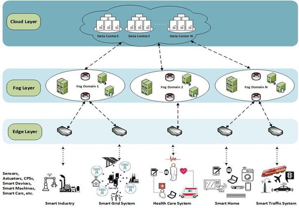
Figure 2.1 Fog Computing Architecture
Fog computing architecture is designed to extend cloud computing capabilities closer to the edge of the network, enabling low-latency data processing and real-time decision-making. This architecture comprises multiple layers, each with distinct roles and responsibilities, facilitating efficient data management and computational task distribution.
Edge Layer:
The edge layer consists of end-user devices and IoT sensors that generate vast amounts of data. These devices, which include smartphones, wearables, industrial sensors, and smart home devices, are the initial data sources. Due to their limited computational and storage capacities, edge devices rely on nearby fog nodes for processing and analysis (Shi et al., 2016). The edge layer is critical for capturing real-time data and providing preliminary processing, such as filtering and aggregation, before transmitting data to higher layers for more intensive processing.
Fog Layer:
The fog layer, also known as the fog node layer, is composed of intermediate computing devices located between the edge devices and the cloud data centers. These devices include gateways, routers, and local servers that possess greater computational and storage resources than edge devices but less than cloud data centers. Fog nodes perform significant data processing tasks, reducing the need to send all data to the cloud, thereby decreasing latency and bandwidth usage (Chiang & Zhang, 2016). This layer is crucial for executing time-sensitive tasks, running local applications, and providing rapid responses to user requests.
Cloud Layer:
The cloud layer consists of centralized data centers that offer extensive computational power, storage capacity, and advanced analytics capabilities. The cloud layer handles large-scale data processing, long-term storage, and complex analytics that are not time-sensitive. It serves as the backbone for data synchronization, large-scale computations, and inter-fog node coordination. While the cloud provides robust processing capabilities, its reliance on centralized infrastructure can introduce latency, making it less suitable for real-time applications (Mouradian et al., 2018).
Communication Layer:
The communication layer underpins the interaction between the edge, fog, and cloud layers. It involves network protocols, connectivity technologies, and communication standards that facilitate data transmission across the different layers. High-speed, low-latency networks, such as 5G and fiber optics, play a pivotal role in ensuring seamless data flow and synchronization between edge devices, fog nodes, and cloud data centers (Jha et al., 2019).
Management and Orchestration Layer:
This layer encompasses the tools and platforms required for managing and orchestrating the distributed resources within the fog architecture. It includes resource allocation, task scheduling, load balancing, and security management. Effective orchestration ensures that computational tasks are distributed optimally across edge devices, fog nodes, and cloud data centers, maximizing resource utilization and maintaining system performance (LE, 2023).
By integrating these layers, fog computing architecture provides a flexible and scalable framework for handling diverse applications that demand low latency, high bandwidth, and real-time processing capabilities. The architecture’s ability to distribute computational tasks efficiently across various layers enhances overall system performance and user experience, making it well-suited for applications in IoT, smart cities, healthcare, and beyond.
Applications of Fog Computing in Different Sectors
Internet of Things (IoT):
Fog computing plays a crucial role in IoT by providing the necessary infrastructure for processing and analyzing data close to the source. This is essential for applications that require real-time decision-making and low latency. For instance, in smart homes, fog nodes can process data from various sensors and devices to control lighting, heating, and security systems efficiently and in real-time (Yi et al., 2015).
Smart Cities:
In smart cities, fog computing enables real-time data processing and analytics for various applications, including traffic management, public safety, and environmental monitoring. By processing data at the edge, fog computing helps reduce latency and bandwidth usage, allowing for quicker responses to traffic congestion, accidents, and other city-wide events (Chiang & Zhang, 2016).
Healthcare:
Fog computing is increasingly used in healthcare for applications that require real-time monitoring and analysis of patient data. For example, wearable devices can continuously monitor patients’ vital signs and transmit data to nearby fog nodes for immediate analysis. This allows healthcare providers to detect and respond to emergencies more quickly and efficiently, improving patient outcomes (Rahmani et al., 2018).
Industrial Automation:
In industrial automation, fog computing supports real-time monitoring and control of manufacturing processes. By processing data locally, fog nodes can quickly detect and respond to anomalies, reducing downtime and improving efficiency. This is particularly important in industries such as oil and gas, where immediate action is required to prevent accidents and ensure safety (Hong & Varghese, 2019).
Transportation:
Fog computing is used in transportation systems to enhance the efficiency and safety of operations. For instance, fog nodes can process data from vehicle sensors, traffic lights, and surveillance cameras to manage traffic flow and reduce congestion. Additionally, fog computing supports the development of autonomous vehicles by providing the low-latency data processing required for real-time decision-making (Zhou et al., 2019).
Retail:
In the retail sector, fog computing can enhance customer experiences and improve operational efficiency. For example, fog nodes can analyze data from in-store sensors to monitor customer behavior and optimize store layouts. Additionally, fog computing can support real-time inventory management by processing data from RFID tags and other tracking technologies, ensuring that products are always available when needed (Naha et al., 2018).
Agriculture:
Fog computing is used in agriculture to support precision farming techniques. By processing data from sensors placed in fields, fog nodes can provide real-time insights into soil conditions, weather patterns, and crop health. This enables farmers to make informed decisions about irrigation, fertilization, and pest control, improving crop yields and reducing resource usage (Bonomi et al., 2012).
The Advantages and Disadvantages of Fog Computing
Advantages
- Reduced Latency:
Fog computing processes data closer to its source, significantly reducing the time required for data to travel to a central server and back. This is essential for applications that require real-time processing, such as autonomous vehicles, industrial automation, and healthcare monitoring (Bonomi et al., 2012).
- Improved Bandwidth Efficiency:
By processing data locally, fog computing reduces the amount of data that needs to be transmitted to the cloud. This helps in managing network bandwidth more efficiently, preventing congestion, and ensuring smoother data flow (Chiang & Zhang, 2016).
- Enhanced Security and Privacy:
Fog computing allows sensitive data to be processed and stored closer to its source, reducing the risk of data breaches during transmission. Localized processing also enables the implementation of security measures tailored to specific environments, enhancing overall data protection (Yi et al., 2015).
- Scalability:
Fog computing supports the seamless addition of new nodes and devices to the network, allowing it to scale efficiently. This scalability is particularly beneficial for growing IoT ecosystems and smart city applications, where the number of connected devices can increase rapidly (Naha et al., 2018).
- Context Awareness:
Fog nodes can be equipped with context-awareness capabilities, allowing them to make intelligent decisions based on the current state of the environment. This leads to more efficient resource allocation and better performance for applications that depend on real-time data (Stojmenovic & Wen, 2014).
- Reliability and Resilience:
Fog computing can improve the reliability and resilience of systems by distributing computational tasks across multiple nodes. In the event of a node failure, other nodes can take over the workload, ensuring continuous operation and reducing the risk of downtime (Hong & Varghese, 2019).
Disadvantages
- Increased Complexity:
Deploying and managing a fog computing infrastructure can be complex due to the need to coordinate multiple distributed nodes. This complexity can increase operational costs and require specialized knowledge for effective management (Chiang & Zhang, 2016).
- Security Challenges:
While fog computing can enhance security by localizing data processing, it also introduces new security challenges. The distributed nature of fog nodes makes them potential targets for cyberattacks, requiring robust security measures to protect each node (Yi et al., 2015).
- Resource Constraints:
Fog nodes, particularly those deployed on edge devices, often have limited computational power and storage capacity compared to centralized cloud servers. This can restrict the types of applications that can be effectively run on fog nodes and necessitate efficient resource management (Naha et al., 2018).
- Maintenance and Updates:
Keeping a distributed fog computing infrastructure up to date with the latest software and security patches can be challenging. Regular maintenance and updates are essential to ensure the system’s reliability and security, adding to the operational burden (Stojmenovic & Wen, 2014).
- Latency Variability:
While fog computing generally reduces latency, the variability in network conditions and the geographical distribution of fog nodes can sometimes lead to inconsistent latency. This variability can affect the performance of latency-sensitive applications (Hong & Varghese, 2019).
- Interoperability Issues:
Integrating fog computing with existing systems and ensuring interoperability between different fog nodes can be problematic. Differences in hardware, software, and communication protocols can create challenges in achieving seamless integration and operation (Naha et al., 2018).
Challenges and Issues Faced In Fog Computing
- Resource Management:
Efficient allocation and utilization of computing, storage, and networking resources across distributed fog nodes (Jain & Kumar, 2021; Naha et al., 2018).
- Security and Privacy Concerns:
Ensuring data integrity, confidentiality, and availability in a distributed and potentially insecure environment (Jain & Kumar, 2021; Naha et al., 2018).
- Scalability:
Ability to handle increasing numbers of devices, applications, and users while maintaining performance and responsiveness (Jha, N., Sheth, A., & Pal, M. ,2019).
- Interoperability:
Seamless communication and integration among heterogeneous devices, platforms, and cloud services (Jain & Kumar, 2021; Naha et al., 2018).
Quality of Experience (QoE) Strategies
Quality of Experience (QoE) is a critical factor in evaluating user satisfaction with IoT applications in fog computing environments. As IoT devices generate real-time data and latency-sensitive applications demand immediate responses, strategies to optimize QoE in fog computing have become increasingly significant. This section explores key strategies for enhancing QoE in fog computing systems tailored to the challenges of IoT applications.
Dynamic Resource Allocation
- Efficient allocation of computational, storage, and networking resources in fog nodes is essential for optimizing QoE.
- Dynamic resource allocation strategies use real-time data analytics and machine learning algorithms to predict workload patterns and adjust resources accordingly (Chen et al., 2020).
- By prioritizing latency-sensitive tasks and distributing less critical tasks across the network, QoE can be improved significantly.
Task Offloading Mechanisms
- Task offloading involves transferring computational tasks from IoT devices to fog nodes or between fog nodes and cloud servers based on processing capabilities and network conditions.
- Adaptive offloading strategies consider QoE metrics such as latency, jitter, and packet loss while ensuring energy-efficient task execution (Jararweh et al., 2016).
- These mechanisms minimize response times and enhance the user experience, especially in applications like real-time video streaming and remote healthcare.
QoE-Centric Scheduling Algorithms
- Scheduling algorithms designed to prioritize tasks based on QoE requirements play a vital role in meeting user expectations.
- QoE-aware schedulers consider factors like task urgency, user preferences, and application sensitivity to delays (Lalitha et al., 2020).
- These algorithms ensure that critical tasks receive higher priority, thereby reducing delays and improving overall satisfaction.
Edge Intelligence Integration
- Integrating artificial intelligence (AI) at the edge enables fog nodes to make intelligent decisions to optimize QoE dynamically.
- Predictive analytics powered by AI can identify potential QoE bottlenecks and take preemptive measures, such as adjusting bandwidth allocation or migrating tasks (Zhao et al., 2021).
- This approach ensures that IoT applications consistently meet user expectations despite varying workloads.
Hybrid Fog-Cloud Models
- Combining fog computing with cloud resources allows applications to leverage the benefits of both paradigms.
- Hybrid models ensure high QoE by offloading less time-sensitive tasks to the cloud while keeping latency-sensitive tasks at the fog level (Mukherjee et al., 2018).
- This strategy balances workload distribution, reduces latency, and enhances overall performance for IoT applications.
Monitoring and Feedback Systems
- Continuous QoE monitoring through end-user feedback and automated metrics collection ensures that the system can adapt to user needs in real-time.
- Feedback mechanisms help identify areas for improvement, allowing fog systems to adjust resource allocation or scheduling strategies to meet QoE goals effectively.
Energy-Aware Strategies
Energy efficiency is a fundamental challenge in fog computing environments due to the limited power resources of fog nodes and the energy-intensive nature of IoT applications. Addressing this issue requires implementing strategies that optimize energy usage without compromising the Quality of Experience (QoE) for end-users. This section explores energy-aware strategies relevant to optimizing IoT applications in fog computing systems.
Dynamic Voltage and Frequency Scaling (DVFS)
- DVFS adjusts the voltage and frequency of processors in fog nodes based on workload demands, reducing energy consumption during periods of low computational activity (Tiwari et al., 2019).
- By scaling down processor performance when full capacity is not required, DVFS minimizes unnecessary power usage while maintaining application performance.
Energy-Efficient Task Scheduling
- Energy-aware scheduling algorithms prioritize task allocation to nodes with optimal energy efficiency, reducing the overall power consumption of the system.
- These algorithms consider factors such as task complexity, execution time, and the energy state of nodes to allocate resources effectively (Gupta et al., 2020).
- Tasks with lower urgency or less critical QoE requirements are often delayed or offloaded to conserve energy.
Workload Consolidation
- Consolidating workloads onto fewer active fog nodes during off-peak hours can significantly reduce energy consumption.
- Idle or underutilized nodes can be switched to low-power states or completely turned off, optimizing energy usage across the network (Kumar et al., 2018).
- This strategy is particularly effective in IoT scenarios with predictable workload patterns.
Energy-Aware Task Offloading
- Task offloading strategies consider the energy constraints of fog nodes, ensuring tasks are directed to nodes or cloud servers with sufficient power resources.
- Offloading decisions are made dynamically, balancing energy efficiency with QoE requirements, such as latency and throughput (Zhang et al., 2021).
- By leveraging both local and remote resources, energy-aware offloading ensures efficient energy utilization.
Green Energy Integration
- Incorporating renewable energy sources, such as solar or wind power, into fog nodes can enhance energy sustainability.
- Fog nodes can prioritize tasks based on the availability of renewable energy, reducing dependency on non-renewable resources (Sharma et al., 2017).
- This approach aligns with sustainability goals and reduces operational costs over time.
Energy-Aware Load Balancing
- Load balancing mechanisms ensure that energy usage is distributed evenly across all active nodes, preventing excessive power drain on specific nodes.
- These mechanisms dynamically redistribute tasks among fog nodes to optimize energy consumption while maintaining QoE for IoT applications (Sun et al., 2019).
Resource Virtualization and Orchestration
- Virtualization technologies enable multiple IoT applications to share the same physical resources, improving energy efficiency by maximizing utilization.
- Orchestration frameworks optimize resource allocation at runtime, ensuring that energy consumption is minimized while meeting application demands (Mejia et al., 2020).
Sleep Scheduling for Fog Nodes
- Nodes can be programmed to enter low-power sleep modes during periods of inactivity or reduced workload.
- Sleep scheduling algorithms determine the optimal times for nodes to switch to and from sleep states, balancing energy savings and service availability (Qin et al., 2021).
Summary of Related Work
| Paper | Problem Discussed | Improved Criteria / Techniques |
| Al Nuaimi et al. (2015) | Fog computing and communication, future directions | – |
| Chiang & Zhang (2016) | Fog computing and IoT research opportunities | – |
| Jain & Kumar (2021) | Task offloading in fog computing, trends, challenges | Current trends, challenges, future directions |
| Jha et al. (2019) | Fog computing, state-of-the-art, challenges | State-of-the-art review, research directions |
| LE (2023) | Fog computing concepts, frameworks, applications | – |
| Mouradian et al. (2018) | Fog computing state-of-the-art, research challenges | Research challenges, advancements |
| Shi et al. (2016) | Edge computing vision, challenges | Vision for edge computing, technical challenges |
| Bonomi et al. (2012) | Fog computing role in IoT | – |
| Hong & Varghese (2019) | Resource management in fog/edge computing | Survey of resource management techniques |
| Naha et al. (2018) | Fog computing trends, architectures, requirements | – |
| Rahmani et al. (2018) | Smart healthcare system using IoT and fog computing | Improved healthcare delivery, IoT integration |
| Yi et al. (2015) | Fog computing concepts, applications, issues | Applications, issues in fog computing |
| Zhou et al. (2019) | Impact evaluation of fog computing on IoT services | Evaluation methodologies, impact assessment |
| Stojmenovic & Wen (2014) | Fog computing scenarios, security issues | Security challenges, scenarios |
| Deb (2001) | Multi-objective optimization using evolutionary algorithms | Multi-objective optimization techniques |
| Goldberg (1989) | Genetic algorithms in search, optimization | Genetic algorithms in optimization |
| Holland (1992) | Adaptation in natural and artificial systems | Adaptation concepts, applications |
| Mnih et al. (2015) | Deep reinforcement learning for control | Deep reinforcement learning applications |
| Sutton & Barto (2018) | Introduction to reinforcement learning | Reinforcement learning basics |
| Lillicrap et al. (2016) | Continuous control with deep reinforcement learning | Continuous control applications |
Chapter Summary and Evaluation
In this chapter, a comprehensive review of the literature on fog computing and related fields was conducted. The literature covered various aspects including the current state-of-the-art, challenges, future directions, and technological advancements in fog computing. Key papers provided insights into the evolving landscape of fog computing, ranging from foundational concepts and frameworks to specific applications and emerging issues. The review highlighted advancements in task offloading strategies and evaluated the impact of fog computing on IoT services. Techniques such as multi-objective optimization and reinforcement learning were explored in the context of improving fog computing systems.
The chapter began with an exploration of foundational concepts and frameworks of fog computing, outlining key contributions and defining the scope of research in the field. It delved into specific applications discussed in seminal works, addressing challenges such as resource management, security concerns, scalability, and interoperability. The literature review underscored the importance of addressing these issues to enhance the efficiency and reliability of fog computing environments. One limitation observed was the varying depth of coverage across different papers, with some focusing more on theoretical frameworks while others provided empirical evaluations or case studies. Additionally, while the literature discussed several techniques and algorithms for optimizing fog computing systems, specific benchmarks and comparative evaluations were not always detailed.
Overall, the chapter synthesized a wide range of perspectives and findings from recent research, providing a solid foundation for understanding the complexities and advancements in fog computing. Future research directions could include more empirical studies, standardized evaluation metrics, and real-world deployment scenarios to further validate theoretical frameworks and enhance practical implementations in fog computing environments.
Methodology and Problem Analysis
The primary goal of this chapter is to analyze the challenges faced and the approaches encountered during the research. By reviewing numerous relevant papers and journals, the causes and issues related to the research topic are further explained. The research objectives will be achieved through techniques such as QoE and energy aware, all of which are explained in detail. Additionally, the chapter presents a framework for the research methodology, including the tools and techniques used for data collection.
Approaches to Research
Research into fog computing focuses on key aspects such as QoE and energy aware. Figure 3.1 illustrates the research methodology framework, indicating that the analysis will focus on computation offloading based on information gathered from literature reviews. The results of this analysis aim to enhance understanding and offer precise insights into challenges affecting the performance of fog computing environments. Additionally, the gathered insights will guide the direction of the research and help formulate specific objectives:
- To provide a QoE-aware application mapping policy to raise user satisfaction.
- To optimize and maintain energy usage at a maximum level through module placement.
- To present a compute offloading technique that prevents fog device overload.
- To obtain the recommended solution and evaluate it against existing methods.

Figure 3.1: Research Methodology Framework
Review Relevant Literature
Numerous academic journals and research papers have been reviewed to explore the interconnections between IoT, cloud computing, and fog computing. The architecture of fog computing, such as its applications in smart cities, smart grids, and eHealth, has been extensively examined to demonstrate its practical value and significance. While most studies emphasize the advantages of fog computing, some delve into critical issues like transmission delays, energy consumption, and security concerns. Additionally, various researchers have proposed approaches, findings, and algorithms addressing these challenges within fog computing. Furthermore, there is ongoing research focusing on task scheduling and resource allocation in fog networks. Insights and experimental outcomes from existing literature will provide valuable support in analyzing problems and methodologies in this research.
Formula Research Problem
Challenges of Developing QoE-aware Application in Fog Computing
Due to the limitations of resources, fog nodes which are situated closer to end users than cloud data centers show observable variations in network round-trip times, data processing speeds, and resource availability. This makes it difficult to place apps in foggy surroundings. In fog, it could be necessary to use multiple application placement policies in order to reach particular service levels. Effective use is already being made of applications that take fog environments’ quality of service (QoS), situational awareness, and resource awareness into account. On the other hand, little study has been done regarding how Quality of Experience (QoE) affects the placement of fog-based applications. In some circumstances, QoE can enhance QoS. Despite being separate policy-based services, QoE and QoS have an impact on one another because of subtle differences.
The concept of Quality of Experience (QoE) pertains to the measuring of numerous service characteristics from a user’s perspective, including tracking their wants, perceptions, and requirements in diverse circumstances. QoE-aware policies can lower churn rates and increase customer loyalty by concentrating on their interests. In fog contexts, these strategies are already in use for resource estimate and service coverage optimization. By utilizing QoE, fog computing may minimize resource consumption, network quality problems, data processing times, and enhance service delivery and recovery. Effective QoE-aware policy development is difficult, nevertheless, because QoE-dominating factors frequently change and user interest in various system functionalities can shift in real-time fog circumstances.
Real-time interactions will predominate over human interventions in the Internet of Things. Therefore, it is not practical to update QoE through regular input. A further challenge for prediction-based QoE models is the wide range of QoE influencing elements. It is challenging to modify placements in response to QoE assessments. After the application is submitted, adjustments must be made in light of reviews. Thus, before putting the application, it is practical to determine the dominating QoE components and their combined impact on user QoE. By assigning applications to the best computer instances based on these parameters, user quality of experience can be enhanced. This makes it possible to monitor how customer satisfaction and QoE change for a given service.
Define Research Objectives
This research has several key objectives. Firstly, it aims to propose a method for computation to prevent overload on fog devices. Also, the research aims to evaluate the proposed solutions and compare their efficiency and performance with existing solutions using collected data.
Proposed QoE-aware Application Mapping Policy
In order to accomplish the first goal of comprehending QoE in connection to its policy, numerous research papers and publications have been studied. With the help of this review, a QoE-aware application mapping policy that shortens data processing times and improves service quality is proposed.
Fuzzy logic-based approaches and multi-constraint single-objective optimization techniques are used in QoE-aware application mapping strategies. QoE can be influenced by a variety of user assumption features, and fog computing instances can be classified according to a number of state criteria characteristics. However, the state criteria in this study are limited to processing time, circulation time, and available resources, while the user assumption criteria are restricted to access rate, necessary resources, and speed.
Compute the Degree of Assumption (DoA) and Capacity Class Grade (CCG) in order to develop a QoE-aware policy. This computation uses the fuzzy logic-based technique since it is the best option because it takes into account the significance of many parameter dominances and the scalability characteristic in different scenarios. The state’s boundaries and the assumption conditions determine how big the corresponding fuzzy sets and rules are scaled.
Multi-constrained single-objective optimization will be used to maximize QoE Gain for application mapping after the DoA of the application mapping request and CCG of fog instances are met. The optimization problem will then be resolved by using an optimization solution with a single target and several constraints.
Developing an Energy-Aware Module Placement
The second goal has been addressed by proposing an energy-aware approach to optimize energy consumption. Reducing execution time, network utilization, and overall energy consumption are the goals of two optimization modules. Energy-conscious approaches are important to understand since they affect the infrastructure’s efficiency and usefulness.
The first module is about placing modules in an energy-conscious manner, which is assigning incoming work or modules to the appropriate fog devices according to their criteria. This module uses two techniques: it determines the MIPS (millions of instructions per second) of the module and the mobile’s lowest energy consumption. To ascertain whether a device can accommodate extra duties or modules, these techniques are contrasted with the fog devices that are now in use. A fog device that can accommodate additional modules is used to receive the incoming module. The next best fog gadget is selected if none are available.
After a mobile device is positioned on a fog device, the second module makes use of dynamic voltage and frequency scaling (DVFS) technology to improve resource utilization and energy consumption. In order to minimize the use of resources and energy, DVFS modifies the MIPS of fog devices to correspond with the needs of the module. Stated differently, after the module is deployed on the fog device, DVFS computes the new MIPS. DVFS modifies the fog device’s MIPS to match the module’s requirements if the incoming module requires less MIPS than the fog device’s capacity.
System Design and Implementation
The proposed techniques are translated into a functional system to achieve all objectives before being deployed as a tool to gather data and user feedback for evaluating their effectiveness. This transformation process involves two main stages: system design and implementation.
In the system design stage, use case diagrams, flowcharts, and pseudocode are utilized to illustrate all activities related to transforming requirements into actionable components. The implementation of the VR game algorithm progresses through three stages. It employs the offloading algorithm to appropriately map modules onto mobile devices, thereby optimizing performance.
During the implementation stage, the methodology is realized using a simulator named iFogSim, which provides a dynamic IoT applications platform for simulations. Eclipse serves as the design and development tool to operate the iFogSim simulator, with the proposed algorithms written in Java programming language. Each component of the proposed systems is meticulously developed and rigorously tested iteratively to achieve predefined objectives.
System Testing and Evaluation
To accomplish the last objective, multiple scenarios have been devised to test the proposed solution alongside a solution without energy-aware considerations. The comparison is based on various aspects, including execution time, total power consumption, and network usage, as revealed by the simulation results. Each scenario analyses a different aspect, leading to unique results that are shown in Table 3.1.
Table 3.1 Arrangement of the fog device and application module in a simulation
| Scenarios | Fog Device arrangement | Application module arrangement | |
| Scenario 1 | Random order of Fog | Increasing Module MIPS | |
| Device MIPS between end user and cloud | requirements from client to last module | ||
| Scenario 2 | Random order of Fog | Decreasing Module MIPS | |
| Device MIPS between end user and cloud | requirements from client to last module | ||
| Scenario 3 | Random order of Fog | Random order of Module | |
| Device MIPS between end user and cloud | MIPS requirements between client and last module | ||
| Scenario 4 | Increasing Fog Device | Increasing Module MIPS | |
| MIPS from end user to cloud | requirements from client to last module | ||
| Scenario 5 | Increasing Fog Device | Decreasing Module MIPS | |
| MIPS from end user to cloud | requirements from client to last module | ||
| Scenario 6 | Increasing Fog Device | Random order of Module | |
| MIPS from end user to cloud | MIPS requirements between client and last module | ||
Following the development phase, the proposed solution is subjected to comparison and evaluation against the existing solution. Data gathering techniques for evaluation and comparison is outlined in Table 3.2. The criteria utilized to assess and compare the proposed and existing solutions include execution time, energy consumption, and network usage.
To conduct the evaluation and obtain results, simulations are carried out using the iFogSim tool. This tool provides a suitable environment for simulating the performance and behavior of the proposed solution in a fog computing context.
The evaluation and comparison process serves as a crucial step in determining the effectiveness and efficiency of the proposed solution. By measuring execution time, energy consumption, and network usage, insights can be gained into the performance improvements achieved by the proposed solution in comparison to the existing solution. The simulation results obtained through this evaluation process will provide valuable data for analyzing the impact and benefits of the proposed solution.
By conducting testing and evaluation, this research aims to validate the advantages and effectiveness of the proposed solution. The comparison with the existing solution will provide a basis for assessing the improvements and contributions made, ultimately demonstrating the feasibility and value of the proposed approach.
Table 3.2 The method employed to collect data for the evaluation and comparison.
| Comparison | Data Gathering technique | Method | Data acquired/gathered |
| Comparison with solution without QoE-aware | Simulation in iFogSim | Quantitative | Comparison result based on energy consumption, execution time and network usage |
| Comparison with solution without energy optimization | Simulation in iFogSim | Quantitative | Comparison result based on energy consumption, execution time and network usage |
| Comparison with solution without computation offloading | Simulation in iFogSim | Quantitative | Comparison result based on energy consumption, execution time and network usage |
| Comparison between solution with QoE-aware | Simulation in iFogSim | Quantitative | Comparison result based on energy consumption, execution time and network usage |
| Comparison between solution with QoE-aware and energy-aware | Simulation in iFogSim | Quantitative | Comparison result based on execution time, network usage and energy consumption |
Documentation
At the conclusion of the research, it is essential to document the steps taken and the findings obtained. This documentation serves as evidence to demonstrate the level of performance and enhancement achieved through the research efforts. It ensures completeness and accuracy in presenting the results to the reader, aiding their understanding of the research flow and the contributions made to existing knowledge. Additionally, thorough documentation will serve as a valuable reference for future researchers in related fields.
Chapter Summary and Evaluation
In conclusion, this research encompasses a thorough problem analysis and methodology discussion. It begins with an examination of the problem statement, offering a detailed exploration of its causes and the issues it presents. A research methodology framework is then developed to guide the achievement of research objectives. Detailed explanations cover topics such as the Computation Offloading Method, System Design and Implementation, System Testing and Evaluation, and Documentation. The research also discusses the tools utiized during the development phase and outlines the data gathering methods employed. The subsequent chapter will delve into the system design and implementation of the proposed solutions.
System Design and Implementation
This chapter will focus on the system design and implementation of the proposed solutions. The solution involves QoE-aware application mapping and energy-aware module placement. The aim is to enhance user satisfaction, minimize execution time, reduce network usage, and optimize energy consumption. The chapter begins with a discussion of the system architecture design, followed by the implementation of QoE-aware application mapping and energy-aware module placement. The chapter concludes with a summary.
System Architecture Design
This section covers the fog computing framework, fog environment simulation, and the modeling of the fog environment and module placement.
The fog computing architecture is built on three layers: the sensor layer, fog layer, and cloud layer. Figure 4.1 illustrates the architecture, which is designed to support the operation of higher layers by assigning specific tasks to each layer.
Service requests from users are gathered in integrated fog and cloud networks. Users are connected to various applications and can send requests to fog nodes via wireless access. The fog nodes process these requests and return the results through the three-layer architecture.
IoT devices linked to applications perform specific functions based on user requests. These devices are divided into multiple interconnected Application Modules for Fog-enabled IoT applications, which include the Client Module and the Main Application Module. The Client Module runs on the user’s proximate devices, handling user preferences, contextual information, and communication with the Main Application Module. The Main Application Module manages all application data operations, producing the final output for the Fog-enabled IoT systems.

Figure 4.1 Fog Computing Architecture
The third layer, the sensor or IoT devices layer, is the closest to the end user. It consists of various IoT devices like sensors, actuators, and mobile phones, which are widely distributed geographically. These devices are modeled as sensors and actuators, capable of emitting data. Sensors detect physical objects or events and transmit the data for processing and storage in the upper layer. Actuators respond to environmental changes based on sensor data.
The second layer, the fog layer, hosts numerous fog nodes, including routers, switches, access points, and fog servers. These nodes are distributed between the cloud center and end devices, providing computing, transmission, temporary storage, and data processing. The fog layer handles real-time analysis and latency-sensitive applications, and connects to the cloud data center via an IP core network. The fog nodes and cloud data centers collaborate to leverage more powerful computing and storage capabilities.
The cloud layer, responsible for global monitoring and control, is located at the top. It includes multiple storage devices and high-performance servers that support extensive computation, long-term data storage, large-scale event detection, and dynamic decision-making. Cloud analytics ensure grid and service vendors can perform large-scale resource management and prepare for power outages.
Three main aspects are considered in fog computing:
Quality of Experience (QoE): QoE is determined by user requirements and perceptions. QoE-aware application mapping is used to enhance data processing time and service quality, employing fuzzy logic and multi-constraint single objective optimization techniques. Fuzzy logic calculates the Degree of Assumption (DoA) and Capacity Class Grade (CCG) for application and computing instances, respectively. These metrics are then optimized to maximize the Rating Gain for application mapping, ensuring a one-to-one mapping between applications and instances.
Energy: Fog Service Placement using Simulated Annealing (FSPSA) optimizes the allocation of services across fog nodes to minimize latency and improve resource efficiency. The process starts by generating an initial random service placement across fog nodes. An energy function evaluates each placement based on factors like latency, resource utilization, and load balancing. FSPSA then explores neighboring solutions by adjusting the service placements, aiming to minimize the energy function. Simulated Annealing allows the algorithm to accept worse solutions with a probability that decreases over time as the temperature lowers, avoiding local optima. The temperature gradually decreases following a cooling schedule until the algorithm converges on an optimal or near-optimal solution. This approach ensures efficient service distribution while balancing fog node resources and maintaining low latency.
Offloading: Offloading in the fog layer involves transferring resource-intensive computational tasks to another fog device due to limitations such as computational power, storage, and energy. An offloading algorithm is proposed to address these challenges, ensuring that when a new task arrives at a fog device, it is offloaded to another device if the current one is already occupied.
In summary, these three aspects are essential for optimizing performance, execution time, and network usage in fog computing environments.
The Distributed Data Flow (DDF) model is created for deployment in fog computing, serving as a role model for applications. Applications with data processing capabilities are modeled as collections of modules that generate useful information based on data output. For instance, output from Module I can be used as input for Module J, creating a data dependency that is represented as a directed graph in this model.
In IoT, sensors serve as the data source, while in cloud architecture, data is known as cloudlets. In fog computing, data is referred to as tuples.
Fog Computing Simulation

Figure 4.2: Main classes
Figure 4.2 shows the main classes in fog environment simulation. Fog controller is one of the physical devices that is responsible for building the fog node to deploy the abstraction, it is similar to cluster lead while also granting communication between cloud and fog layers. The Controller is used to control the ModuleMapping, FogDevice as well as the Application.
QoE is used to support module mapping in order to develop an QoE-aware application mapping policy which improves overall user experience and ensures one to one mapping between applications and instances. The second process will be gone through in Energy class which is an energy-aware module placement after application being mapped to fog instance. Energy-aware module placement aims to optimise the energy consumption as well as execution time and usage of the network. Next, the Offloading class is to prevent the overloading of a fog device through the implementation of a proposed offloading algorithm. Through this algorithm, the task will be offloaded to other fog nodes instead of executing when the current fog device is processing a task. After these three processes, the results will be passed to ModulePlacementMapping and finally the module is placed to the suitable fog device by ModulePlacement class. The results will be returned back to application after the task is processed by the fog device. The three classes which are AppModule, AppLoop and AppEdge connect to the application. AppModule serves as the processing elements of fog applications. AppModule will process and send the generated output tuples to next modules in the DAG. AppLoop is an extra class, utilised for determining the loops that are important to the user and controls the process whereas an AppEdge case indicates the information reliance between a couple of application modules and represents a directed edge in the application mode.
Modeling Fog Environment
The target application is a fog computing environment that consists of multiple fog devices which can bring the cloud applications closer to the physical IoT devices at the network edge. Fog device is also known as fog node which is able to process tuples that were sent from other modules hosted on the other fog node hence qualifying fog node as a “mini-cloud” located at the edge of a network that is interconnected by varieties of communication technologies. Virtual machine is the logical data flow presented in a physical fog node in order to fully leverage the processing capability of the fog node. Thus, the virtual machine which is located in the fog devices will process the tuple according to the tuple scheduler. A host is a computer or other device that communicates with other hosts on a network. Hosts on a network include clients and servers that send or receive data, services or applications. Based on research, only one application module is provisioned within a single virtual machine instance to simplify the testing. Figure 4.3 shows the relationship of the related main entities of the proposed solution.

Figure 4.3: The relationship of the main entities in proposed solution
Application is composed of modules that could be individually hosted on fog nodes to fully leverage the potential of fog devices. The characteristics of modules include maximum MIPS requirement, RAM requirement, Bandwidth requirement, and the tuple frequency. On the other hand, the characteristics of fog devices include MIPS, RAM, bandwidth, link latency, and energy consumption.
iFogSim supports resource management service through two application module placement. “Cloud-only placement” is all modules of an application run in data centres whereas “Edgeward placement” is application modules that are placed close to the edge of the network. However, devices close to the edge of the network may not be powerful enough to host all the applications. The placement policy determines how application modules are placed across Fog devices upon submission of application. The placement process can be driven by objectives such as minimising end-to-end latency, network usage, operational cost, or energy consumption. The class Module Placement is the abstract placement policy that needs to be extended for integrating new policies. The illustration of module placement is shown in Figure 4.4.

Figure 4.4: Illustration of module placement
QoE-aware Application Mapping
QoE-aware application will be the first process in phase one of a proposed solution which enhances the user satisfaction.
Architecture of QoE-aware Application Mapping
The computational nodes are equipped with resources such as memory, bandwidth and CPU to run various applications for computational fog nodes (CFN). The resources are virtualized among MSs, micro services, where assignment of applications for execution are conducted in computational nodes. Dynamic provision on the additional resources for a micro service can be conducted from either In CFN, all configured MSs can be operated independently. Controller node is in charge of monitoring and controlling the overall activities of CFN. There is data storage in the controller node that stores metadata that is related to the running application and State Criteria parameters of the MSs. In the controller node, a Capacity Grade Unit is proposed to define a capacity index for each MS based on the State Criteria parameters to ensure that MSs are ranked in accordance with their competence.
Sometimes, the computation of data signals transmitted from IoT devices is facilitated by edge fog nodes, EFNs. For certain Fog-enabled IoT systems, it is assumed that the corresponding EFNs run the Client Module and aid in placing the subsequent module to CFNs in the upper level. In this approach, the connections are established between EFNs and IoT devices. The Client Module is initiated by the Application Initiation Unit of EFNs, through which a user expresses assumptions related to the application to EFNs. EFN services are used to obtain and collect the capacity index of MSs and it is stored in a data storage. Moreover, the data storage keeps user Assumption Criteria and Quantity of Service (QoS) attributes related to the application for further processing. In EFN, there are two individual units which are, Application Mapping Unit and Assumption Degree Unit. For each application mapping request, Assumption Degree Unit calculates a priority value by considering user Assumption Criteria. Other than that, the Application Mapping Unit of EFN carries out mapping of applications to appropriate Fog instances according to the priority value of application mapping requests and the capacity index of MSs respectively. Figure 4.5 shows the architecture for QoE-aware application mapping.

Figure 4.5: Architecture for QoE-aware application mapping
Flow of QoE-aware Application Mapping
The calculation of a priority value called Degree of Assumption (DoA) will be the essential steps of each application mapping request according to the user assumption parameters, and also to calculate a capacity index called Capacity Class Grade (CCG) of MSs in CFNs in accordance to the state parameters and guarantee the QoE maximised applications mapping to competent MSs using DoA and CCG values. It requires the active participation of Assumption Degree Unit, Application Mapping Units of EFNs and Capacity Grade Unit of CFNs in order to carry out the steps. Figure 4.6 shows the sequence diagram for QoE-aware application mapping.

Figure 4.6: Sequence diagram for QoE-aware application mapping
To ensure the best quality of experience for end users, the calculation of two values is vital. The two values are DoA of an application and CCG of a computing instance to effectively map the application to fog instances. There are several steps that need to be followed from the calculation of two values until mapping of application. The first step is to get the Bandwidth, Demanded Resources and Latency Acceptability to store into data storage from the clients assumption. The parameters are sent for DoA calculation through the process of fuzzy inference and defuzzification after assumption parameters are normalised. After calculating DoA, edge fog nodes will query the accessibility of cloud fog nodes about available micro services and CCG values will be associated. Then, State Criteria will be acquired for the calculation of CCG and the CCG is sent once it is calculated. The total Rating Gain of the applications are maximised in the process of mapping applications on that instance. QoE-aware mapping of the applications will be promoted based on the maximum Rating Gain.
Notation and Definition
Table 4.1 shows the QoE-aware application mapping notations and definitions.
Table 4.1: Notations for QoE-aware application mapping
|
Symbol |
Definition |
|
|
Set of all Edge Fog Nodes (EFNs) |
|
|
Set of all Computational Fog Nodes (CFNs) |
|
|
Degree of Assumption ( |
|
|
Capacity Class Grade ( |
|
|
Set of all application mapping request in EFN |
|
|
Set of all micro services in CFN |
|
|
Bandwidth parameter in Assumption Criteria |
|
|
Demanded resources parameter in Assumption Criteria |
|
|
Latency Acceptability parameter in Assumption Criteria |
|
|
Circulation time parameter in State Criteria |
|
|
Resource availability parameter in State Criteria |
|
|
Processing speed parameter in State Criteria |
|
|
Assumption Criteria for application |
|
|
State Criteria for instances |
|
|
DoA of application |
|
|
Data signal size for |
|
|
CCG of instances |
|
|
Assumption (value) of parameter ω for application |
|
|
State (value) of parameter ɛ for instances |
|
|
Fuzzy membership function for any |
|
|
Fuzzy membership function for any |
|
|
Fuzzy outcome set for DoA calculation. |
|
|
Fuzzy outcome set for CCG calculation. |
|
|
Singleton value for a Fuzzy outcome in (DoA) |
|
|
Singleton value for Fuzzy outcome in (CCG) |
|
|
Membership function for any Fuzzy outcome in DoA calculation |
|
|
Membership function for any Fuzzy outcome in CCG calculation |
|
|
Equals to 1 if |
|
|
Normalised access rate |
|
|
Normalised resource requirement |
|
|
Normalised processing time |
|
|
Fuzzification bandwidth set |
|
|
Fuzzification resource requirement set |
|
|
Fuzzification processing time set |
|
|
Fuzzification Inference |
|
|
Defuzzification Singleton |
|
s |
Singleton |
|
|
Defuzzification |
|
RoE |
Return on Equity Value |
|
CCS |
Cloud Computing and Services Value |
Calculation of Degree of Assumption (DoA)
Based on the specific fog environment, application placement requests are given distinctive expectation parameters‘ range. The amount of the parameter can be chosen unless it didn’t reach beyond the range.
Table 4.2: Range of the Parameters for DoA
|
Parameter/Metrics |
Value in Range |
|
Bandwidth |
(3, 18) |
|
Demanded Resources |
(4, 16) |
|
Latency Acceptability |
(20, 140) |
The users end device compromise to the ![]() regarding an application
regarding an application ![]() to the system through the Application Initiation Unit. The data storage will contain the
to the system through the Application Initiation Unit. The data storage will contain the ![]() and it is sent to the Assumption Degree unit of EFN
and it is sent to the Assumption Degree unit of EFN ![]() .
. ![]() which contain three parameters and the range. The units of the values vary. The values of each parameter are normalised to simplify further calculation. The result of the normalisation will fall in between -1 and 1 by using Eq.4.1:
which contain three parameters and the range. The units of the values vary. The values of each parameter are normalised to simplify further calculation. The result of the normalisation will fall in between -1 and 1 by using Eq.4.1:
|
|
(4.1) |
![]() is the normalised value for criteria
is the normalised value for criteria ![]() within the range
within the range ![]() . Each criteria in
. Each criteria in ![]() , is defined based on the scope for every criteria of Table 4.2 offered in the Fog Environment. In the other words,
, is defined based on the scope for every criteria of Table 4.2 offered in the Fog Environment. In the other words, ![]() refer to the minimum value of the range of parameters,
refer to the minimum value of the range of parameters, ![]() refers to maximum value of the range of parameters In Assumption Degree Unit, a Fuzzy logic based approach is used to calculate the
refers to maximum value of the range of parameters In Assumption Degree Unit, a Fuzzy logic based approach is used to calculate the ![]() of each application from the normalised parameter in
of each application from the normalised parameter in ![]() .
.
Fuzzification Module for DoA Calculation
Fuzzification is used to convert the crisp input values into fuzzy values by using the information in the knowledge base. In fuzzification, the crisp inputs which are x and y are taken to determine the degree whether they belong to which of the appropriate fuzzy sets. The standardised value ![]() of any
of any ![]() parameter
parameter ![]() is transformed into an equivalent fuzzy dimension through associate membership function
is transformed into an equivalent fuzzy dimension through associate membership function![]() . This work involved membership functions of different Assumption Criteria from three different fuzzy sets. The following are the fuzzy sets:
. This work involved membership functions of different Assumption Criteria from three different fuzzy sets. The following are the fuzzy sets:
● Bandwidth: ![]()
● Demanded resources: ![]()
● Latency Acceptability: ![]()
In this case, the following ![]() value will be given as 6 per seconds, 7 CPU cores and 110 ms to Bandwidth, Demanded Resources and Latency Acceptability respectively, as shown in Table 4.3.
value will be given as 6 per seconds, 7 CPU cores and 110 ms to Bandwidth, Demanded Resources and Latency Acceptability respectively, as shown in Table 4.3.
Table 4.3 Value of DoA Calculation
|
Parameter |
Bandwidth (per seconds) |
Demanded Resource (CPU cores) |
Latency Acceptability (ms) |
|
|
3 |
4 |
20 |
|
|
18 |
16 |
115 |
|
|
6 |
7 |
100 |
After the value is prepared, it takes fuzzy input and applies it to the antecedents of fuzzy rules, then it can start to calculate the Degree of Assumption (DoA) as shown in Table 4.4 based on Eq.4.1:
Table 4.4: Result of Calculation of DoA
|
Bandwidth |
Demanded Resource |
Latency Acceptability |
|
|
|
|
The membership degree, ![]() for any normalised value for criteria
for any normalised value for criteria ![]() based on respective fuzzy sets in Figure 4.7. Table 4.5 is fuzzy sets after assumption parameters that are normalised. The fuzzy set will be arranged in:
based on respective fuzzy sets in Figure 4.7. Table 4.5 is fuzzy sets after assumption parameters that are normalised. The fuzzy set will be arranged in:
❖ Bandwidth:
➢ ![]()
❖ Demanded Resource:
➢ ![]()
❖ Latency Acceptability:
➢ ![]()

Figure 4.7: Membership function of assumption criteria parameters
Before the normalisation process, it is assumed that the value of parameter ![]() in application. Fuzzy sets can be displayed in many shapes. However, triangles or trapezoids can usually fully express expert knowledge and can greatly simplify the calculation process. Figure 4.8 shows how Fuzzy logic separates the area for Bandwidth fuzzy sets.
in application. Fuzzy sets can be displayed in many shapes. However, triangles or trapezoids can usually fully express expert knowledge and can greatly simplify the calculation process. Figure 4.8 shows how Fuzzy logic separates the area for Bandwidth fuzzy sets.

Figure 4.8: Area separation for Bandwidth fuzzy sets
After the normalisation process is complete in Table 4.4, the answer for ![]() is = -0.60.
is = -0.60. ![]() refer to the normalised application 1 under Bandwidth parameter
refer to the normalised application 1 under Bandwidth parameter ![]() . Based on the result, it is shown that -0.60 of the x axis hit 0.5 on the y axis of its respective membership set in the Extremely Low and Low area. Refer Figure 4.9, therefore it is concluded that the fuzzy set for
. Based on the result, it is shown that -0.60 of the x axis hit 0.5 on the y axis of its respective membership set in the Extremely Low and Low area. Refer Figure 4.9, therefore it is concluded that the fuzzy set for ![]() .
.

Figure 4.9: Bandwidth normalised value intercepted Extremely Low and Low area
In parameter of Demanded Resources, ![]() is = -0.50.
is = -0.50. ![]() refer to the normalised application 1 under Demanded Resources parameter
refer to the normalised application 1 under Demanded Resources parameter ![]() . Based on the result, it is shown that -0.50 of x axis hit 0.65 and 0.35 on y axis in Small and Medium area on y-axis of its respective membership set correspondingly, therefore it is concluded that the fuzzy set for
. Based on the result, it is shown that -0.50 of x axis hit 0.65 and 0.35 on y axis in Small and Medium area on y-axis of its respective membership set correspondingly, therefore it is concluded that the fuzzy set for ![]() .
.
In parameter of Latency Acceptable, ![]() is = 0.50.
is = 0.50. ![]() refer to the normalised application 1 under Latency Acceptability parameter
refer to the normalised application 1 under Latency Acceptability parameter ![]() . Based on the result, it is shown that 0.50 of x axis hit 0.35 and 0.65 on y axis in Moderate and High membership sets respectively, therefore it is concluded that the fuzzy set for
. Based on the result, it is shown that 0.50 of x axis hit 0.35 and 0.65 on y axis in Moderate and High membership sets respectively, therefore it is concluded that the fuzzy set for ![]() . Table 4.5 shows the examples of fuzzy sets after assumption parameters being normalised.
. Table 4.5 shows the examples of fuzzy sets after assumption parameters being normalised.
Table 4.5: Fuzzy sets after assumption parameters being normalised
|
Parameter |
DoA ( |
Intercepted Area of Y-axis (Normalised Value) |
|
||||
|
Bw |
-0.60
|
Extremely Low (0.50) |
Low (0.50) |
Medium (0.00) |
High (0.00) |
Extremely High (0.00) |
{0.50,0.50,0.00,0.00,0.00} |
|
Dr |
-0.50 |
|
Small (0.65) |
Medium (0.35) |
Large (0.00) |
|
{0.65,0.35,0.00} |
|
La |
0.77 |
|
Slow (0.00) |
Moderate (0.35) |
Fast (0.65) |
|
{0.00,0.35,0.65} |
Fuzzy Inference Module for DoA Calculation
Fuzzy inference is used to formulate a mapping from a given input to an output using fuzzy logic. Then, the mapping will provide the basis from which decisions can be made or patterns can be identified. During fuzzy inference, corresponding fuzzy outputs are determined by mutually comparing fuzzy inputs with the help of fuzzy rules. The fuzzy rules are set in such a way that approximately stringent assumption parameters like large resource demand are given higher weight. As a result, the DoA value for the requests will be more aligned with the stringent assumption parameters compared to flexible parameters like moderate latency acceptable and medium bandwidth. After that, the system needs to be tuned and evaluated to see if the fuzzy system meets the requirements specified at the beginning. The surfaces can be generated by using the fuzzy logic toolbox to analyse the performance of the system. The fuzzy rules used to calculate DoA are shown in Figure 4.10 while the results of fuzzy inputs (Assumption Criteria parameters) comparison based on the fuzzy rules are shown in Appendices.

Figure 4.10: Fuzzy rules for DoA calculation
The membership degree for each of the fuzzy outputs refers to the highest membership degree of each compared parameter from the corresponding fuzzy set. The figure 4.10 is based on table 4.2 Range of the Parameters for DoA. The equation used to determine the membership degree is shown in Eq.4.2:
|
|
(4.2) |

Figure 4.11: Fuzzy rules for DoA calculation
From Figure 4.11, the bandwidth will be divided into 5 types which are ‘EH’, ‘H’, ‘M’, ‘L’, ‘EL’ and represent ‘Extremely High’, ‘High’, ‘Medium’, ‘Low’ and ‘Extremely Low’. The resource demand is divided into 3 types which are ‘L’, ‘M’, ‘S’ and represent ‘Large’, ‘Medium’, ‘Small’. Using the comparison of the first fuzzy set as an example, with the Extremely Low Bandwidth, Small Demanded Resource and Low Latency Acceptance, the fuzzy output will be on an Extremely High level. The illustrative explanation is shown in Figure 4.11. From Figure 4.11, the bandwidth will be divided into 5 types which are ‘EH’, ‘H’, ‘M’, ‘L’, ‘EL’ and represent ‘Extremely High’, ‘High’, ‘Medium’, ‘Low’ and ‘Extremely Low’. The resource demand is divided into 3 types which are ‘L’, ‘M’, ‘S’ and represent ‘Large’, ‘Medium’, ‘Small’. Using the comparison of the first fuzzy set as an example, with the Extremely Low Bandwidth, Small Demanded Resource and Low Latency Acceptance, the fuzzy output will be on an Extremely High level. The illustrative explanation is shown in Figure 4.12. Any u number of fuzzy rules can be triggered based on the Assumption Criteria parameters.

Figure 4.12: Illustrative explanation on getting fuzzy output for DoA calculation
Defuzzification Module of DoA calculation
The maximum rating of the application for that fuzzy output is represented by a value called singleton value which is set in a way that could make the logical difference on having fuzzy outputs obviously visible. In this case, the singleton value for fuzzy output is set as ‘Extremely High’, ‘High’, ‘Medium’, ‘Low’ and ‘Extremely Low’ as 10, 8, 6, 4 and 2 respectively. Fuzziness helps us evaluate the rules, but the final output of the fuzzy system must be a clear number. The input of the defuzzification process is the aggregate output fuzzy set, and the output is a single number. For defuzzification, Fuzzy logic is applied on different parameters of the Assumption Criteria to obtain the exact DoA for application. The equation used to obtain DoA is shown in Eq.4.3:
 (4.3)
(4.3)
Each membership degree will be multiplied with the corresponding singleton value, then all the values resulted from the multiplication will be summed up and lastly, be divided by the sum of all membership degrees. ![]() refers to the exact DoA obtained for application
refers to the exact DoA obtained for application ![]() . The Application Mapping Unit will then use
. The Application Mapping Unit will then use ![]() to map the application to a suitable Fog computing instance.
to map the application to a suitable Fog computing instance.
Calculation of Capacity Class Grade (CCG)
Table 4.6: Range of the Parameters for CCG
|
Parameter/Metrics |
Value in Range |
|
Circulation Time |
(2, 17) |
|
Available Resources |
(3, 15) |
|
Processing Time |
(40, 160) |
CCG is calculated after the calculation of DoA has been done for each application placement request. At this stage, EFN ![]() will question the accessibility of CFN
will question the accessibility of CFN ![]() on the available micro services
on the available micro services ![]() and associate CCG values. For every micro services in a CFN, the CCG is calculated in Capacity Class Grading unit from the correlated State Criteria,
and associate CCG values. For every micro services in a CFN, the CCG is calculated in Capacity Class Grading unit from the correlated State Criteria, ![]() . The calculation steps are similar to calculation for Degree of Assumption (DoA). The values for State Criteria parameters are different, therefore the normalisation process is carried out using Eq.4.4:
. The calculation steps are similar to calculation for Degree of Assumption (DoA). The values for State Criteria parameters are different, therefore the normalisation process is carried out using Eq.4.4:
|
|
(4.4) |
![]() is the result after the normalisation process for criteria
is the result after the normalisation process for criteria ![]() within the range
within the range ![]() . The range is set based on the capacity of the Fog environment for those respective parameters. After normalisation, a Fuzzy logic based approach is used for further calculation.
. The range is set based on the capacity of the Fog environment for those respective parameters. After normalisation, a Fuzzy logic based approach is used for further calculation.
Fuzzification Module for CCG Calculation
The membership ![]() is use to determine the membership degree of normalised
is use to determine the membership degree of normalised ![]() value to relate fuzzy sets. This fuzzy sets for each parameter are listed as follow:
value to relate fuzzy sets. This fuzzy sets for each parameter are listed as follow:
- Circulation time:

- Resource Availability:

- Processing Time:

In this case, the following ![]() value will be given a sample as 11 per seconds, 12 CPU cores and 85 ms to Circulation Time, Resources Availability and Processing Time respectively, as shown in Table 4.7.
value will be given a sample as 11 per seconds, 12 CPU cores and 85 ms to Circulation Time, Resources Availability and Processing Time respectively, as shown in Table 4.7.
Table 4.7 Value of CCG Calculation
|
Parameter |
Circulation Time (per seconds) |
Resource Availability (CPU cores) |
Processing Time (ms) |
|
|
2 |
3 |
40 |
|
|
17 |
15 |
160 |
|
|
11 |
12 |
85 |
After the value is prepared, calculate the Capacity Class Grade (CCG) as shown in Table 4.8 based on Eq.4.4:
Table 4.8: Result of Calculation of CCG
|
Circulation Time |
Resources Availability |
Processing Time |
|
|
|
|
The membership function, ![]() for state criteria parameters is shown in Figure 4.13, while examples of fuzzy sets after state parameters that are normalised are shown in Table 4.9. The fuzzy set will be arranged in:
for state criteria parameters is shown in Figure 4.13, while examples of fuzzy sets after state parameters that are normalised are shown in Table 4.9. The fuzzy set will be arranged in:
❖ Bandwidth:
➢ ![]()
❖ Demanded Resources:
➢ ![]()
❖ Latency Acceptability:
➢ ![]()

Figure 4.13: Membership function of state criteria parameters
After the normalisation process is complete in Table 4.8, the answer for Circulation Time, ![]() is = 0.20.
is = 0.20. ![]() refer to the normalised application 1 under Bandwidth parameter
refer to the normalised application 1 under Bandwidth parameter ![]() . Based on the result, it is shown that 0.20 of x axis hit 0.5 on y axis of its respective membership set in Average and Long area, therefore it is concluded that the fuzzy set for
. Based on the result, it is shown that 0.20 of x axis hit 0.5 on y axis of its respective membership set in Average and Long area, therefore it is concluded that the fuzzy set for ![]() .
.
In parameter of Resource Acceptability, ![]() is = 0.50.
is = 0.50. ![]() refer to the normalised application 1 under Demanded Resources parameter
refer to the normalised application 1 under Demanded Resources parameter ![]() . Based on the result, it is shown that 0.50 of x axis hit 0.35 and 0.65 on y axis in Adequate and Sufficient area on y-axis of its respective membership set correspondingly, therefore it is concluded that the fuzzy set for
. Based on the result, it is shown that 0.50 of x axis hit 0.35 and 0.65 on y axis in Adequate and Sufficient area on y-axis of its respective membership set correspondingly, therefore it is concluded that the fuzzy set for ![]() .
.
In parameter of Processing Time, ![]() is = -0.25.
is = -0.25. ![]() refer to the normalised application 1 under Latency Acceptability parameter
refer to the normalised application 1 under Latency Acceptability parameter ![]() . Based on the result, it is shown that -0.25 of x axis hit 0.35 and 0.65 on y axis in Minimal and Fair membership sets respectively, therefore it is concluded that the fuzzy set for
. Based on the result, it is shown that -0.25 of x axis hit 0.35 and 0.65 on y axis in Minimal and Fair membership sets respectively, therefore it is concluded that the fuzzy set for ![]() .
.
Table 4.9: Fuzzy sets after state parameters being normalised
|
Parameter |
CCG ( |
Intercepted Area of Y-axis (Normalised Value) |
|
||||
|
Ct |
0.20 |
Extremely Short (0.00) |
Short (0.00) |
Average (0.50) |
Long (0.50) |
Extremely Long (0.00) |
{0.0,0.0,0.5,05,0.00} |
|
Ra |
0.50 |
|
Limited (0.00) |
Adequate(0.35) |
Sufficient (0.65) |
|
{0.00,0.35,0.65} |
|
Pt |
-0.25 |
|
Minimal (0.35) |
Fair (0.65) |
Optimal (0.00) |
|
{0.35,0.65,0.00} |
Fuzzy Inference Module for CCG Calculation
Corresponding fuzzy outputs are determined by mutually comparing fuzzy inputs with the help of fuzzy rules during fuzzy inference similar to the calculation of DoA. However, the fuzzy rules for calculating CCG give higher weight to those approximately impediment state parameters such as long Circulation Time. As a result, the CCG value of the instances indicate more on the limitation instead of the convenience such as adequate Resources Availability and fair Processing Time. The fuzzy rules used to calculate CCG are shown in Figure 4.14 which is based on table 4.6, while the results of fuzzy inputs comparison based on the fuzzy rules are shown in Appendices.

Figure 4.14: Fuzzy rules for CCG calculation

Figure 4.15: Fuzzy rules for CCG calculation
From Figure 4.15, the calculation time will be divided into 5 types which are ‘ES’, ‘S’, ‘A’, ‘L’, ‘EL’ and represent ‘Extremely Short’, ‘Short’, ‘Average’, ‘Long’ and ‘Extremely Long’. The resource availability is divided into three types which are ‘S’, ‘A’, ‘L’ and represent ‘Sufficient’, ‘Adequate’, ‘Limited’. The membership degree for each of the fuzzy outputs refers to the lowest membership degree of the compared parameters from the corresponding fuzzy set. The equation used to determine the membership degree is shown in Eq.4.5:
![]() (4.5)
(4.5)
Using the result of the comparison of the first fuzzy set as a reference, with the short Circulation Time, limited Resources Available and minimal Processing Time, the fuzzy output will be Lower. The illustrative explanation is shown in Figure 4.16.


Figure 4.16: Illustrative explanation on getting fuzzy output for CCG calculation
Defuzzification Module for CCG Calculation
In this case, the singleton value represents the maximum rating of the application for that fuzzy output. The singleton values for fuzzy output are set as ‘Extremely High’, ‘High’, ‘Medium’, ‘Low’ and ‘Extremely Low’ as 10, 8, 6, 4 and 2 respectively. For defuzzification, the membership degrees generated are combined with an equation to obtain the exact CCG, ![]() of the instance. The equation used to obtain CCG is shown in Eq.4.6:
of the instance. The equation used to obtain CCG is shown in Eq.4.6:
 (4.6)
(4.6)
Each membership degree will be multiplied with the corresponding singleton value, then all of the values resulting from the multiplication will be summed up and lastly be divided by the sum of all membership degrees. The CCG obtained is then forwarded to the querying EFN to carry out the following application mapping process.
Application Mapping to Fog Instances
The output of DoA of an application and CCG of a computing instance is named Rating Gain for mapping the application on that instance. The total Rating Gain of the applications are maximised in the process of mapping applications to computing instances. The maximum Rating Gain is able to promote the QoE-aware mapping of the applications. The high combined intensity of associate Assumption Criteria parameters are denoted by the high DoA of the applications. The higher CCG relatively indicates better ability of the instances to satisfy different user assumptions even within the weaknesses. DoA of an application serves as the representative parameter for all of its assumption parameters, therefore the best possible convergence of the assumption parameters to corresponding state parameters of the instances are guaranteed by the maximised Rating Gain of the particular application. As a result, the chance of managing Fog facilities such as computational resources and service accessibility increases without affecting the user assumptions, the QoE regarding the applications are optimised as well.
In an EFN, the applications are mapped to computing instances in the Application mapping unit using a multi-constraint objective function. The multi-constraint objective function is shown in Eq.4.7:
 (4.7)
(4.7)
Throughout the objective function, the Rating Gain for all application mapping requests are maximised to improve overall user QoE, one to one mapping between applications and instances are guaranteed, and the QoS of the application including service delivery time, service cost and packet loss rate are maintained. In case mapping that satisfies the constraints is not arranged by the EFN, the nodes will be queried for further instances.
The objective function satisfied the decentralised optimization problem. The optimization problem will be solved and the application will be mapped once the application mapping requests are submitted to an EFN. The EFN can solve this optimization problem with multiple constraints using any integer programming solver such as SCIP. A local view of the Fog system is considered by EFN in order to solve the optimization problem. Due to the location, the chance for an EFN to receive a huge load of application mapping requests in a specific time is low. Thus, the optimization problem is less likely to be an NP-hard problem.
Algorithm for QoE-aware Application Mapping
The pseudocode for QoE-aware application mapping is presented in Figure 4.17:
Algorithm 1 QoE-Aware Application Mapping
1: function DoA(bandwidth, demandedResources, latencyAcceptability)
2: ![]() = bandwidth ← Normalised bandwidth within (-1, 1)
= bandwidth ← Normalised bandwidth within (-1, 1)
3: ![]() = demandedResources ← Normalised demanded resources within (-1,1)
= demandedResources ← Normalised demanded resources within (-1,1)
4: ![]() = latencyAcceptability ← Normalised latency acceptability within (-1, 1)
= latencyAcceptability ← Normalised latency acceptability within (-1, 1)
5: ![]() =
= ![]() ← convert Normalised Bw to fuzzy set
← convert Normalised Bw to fuzzy set
6: ![]() =
= ![]() ← convert NormalisedRR to fuzzy set
← convert NormalisedRR to fuzzy set
7: ![]() =
= ![]() ← convert NormalisedPT to fuzzy set
← convert NormalisedPT to fuzzy set
8: for each ![]() = min..max do
= min..max do
9: for each ![]() = min..max do
= min..max do
10: for each ![]() = min..max do
= min..max do
11: take the largest among the 3 values then
12: store in ![]()
13: ![]() +=
+= ![]() * s
* s
14: ![]() +=
+= ![]()
15: end
16: end
17: end
18: return DoA = ![]() /
/![]()
19 end function
20: function CCG(circulationTime, availableRequirement, processingTime)
21: ![]() = circulationTime ← Normalised circulation time within (-1, 1)
= circulationTime ← Normalised circulation time within (-1, 1)
22: ![]() = availableRequirement ← Normalised available requirement within (-1,1)
= availableRequirement ← Normalised available requirement within (-1,1)
23: ![]() = processingTime ← Normalised processing time within (-1, 1)
= processingTime ← Normalised processing time within (-1, 1)
24: ![]() =
= ![]() ← convert Normalised to fuzzy set
← convert Normalised to fuzzy set
25: ![]() =
= ![]() ← convert NormalisedRR to fuzzy set
← convert NormalisedRR to fuzzy set
26: ![]() =
= ![]() ← convert NormalisedPT to fuzzy set
← convert NormalisedPT to fuzzy set
27: for each![]() = min..max do
= min..max do
28: for each ![]() = min..max do
= min..max do
29: for each![]() = min..max do
= min..max do
30: take the smallest among the 3 values then
31: store in ![]()
32: ![]() +=
+=![]() * s
* s
33: ![]() +=
+= ![]()
34: end
35: end
36: end
37: return CCG = ![]() /
/![]()
38 end function
Figure 4.17: Pseudocode for QoE-aware application mapping
System Testing for QoE-aware Application Mapping
A policy called Edgeward is implemented in the fog simulator and used as comparison to our proposed solution. Edgeward placement strategy is inclined towards the deployment of application modules close to the edge of the network. However, devices close to the edge of the network may not be computationally powerful enough to host all operators of the application. In such a situation, the strategy iterates on fog devices towards clouds and tries to place remaining operators on alternative devices.
This section is to ensure the validation testing is verifying every class in the iFogSim simulation to be accurate and properly running. Table 4.10 shows some of the simulation parameters which include processing capacity of fog devices, RAM of fog devices, network latency, fog device upstream and downstream capability, module size and tuple size.
Table 4.10: Simulation parameters for QoE-aware application mapping testing
| Parameter | Value |
| Processing capacity of fog devices | 500 – 4500 MIPS |
| RAM of fog devices | 200 – 1800 Mb |
| Network latency | 2 – 100 ms |
| Fog Device Upstream capability | 1024000 Mbps |
| Fog Device Downstream capability | 1024000 Mbps |
| Module Size | 150 – 1100 MIPS |
| Tuple Size | 100 – 3000 MIPS |
Before the comparison between the proposed solutions with others’ work is carried out, few scenarios are defined to have an accurate result. In the simulation, few aspects are compared which are the execution time, total power consumption and total network usage. Different aspects will display different results which depend on the scenario. Table 4.11 shows the 6 scenarios used to simulate the results of the proposed solution. All the scenarios are using 1 application to run.
Table 4.11: Simulation scenarios used in the experiments
| Scenario | Fog Device Arrangement | Application Module Arrangement |
| Scenario 1 | Fog Device MIPS increases from end user towards cloud | Module’s MIPS requirements increases from client towards last module |
| Scenario 2 | Fog Device MIPS increases from end user towards cloud | Module’s MIPS requirements decreases from client towards last module |
| Scenario 3 | Fog Device MIPS increases from end user towards cloud | Module’s MIPS requirements is in random order between client and last module |
| Scenario 4 | Fog Device MIPS is in random order between end user and cloud | Module’s MIPS requirements increases from client towards last module |
| Scenario 5 | Fog Device MIPS is in random order between end user and cloud | Module’s MIPS requirements decreases from client towards last module |
| Scenario 6 | Fog Device MIPS is in random order between end user and cloud | Module’s MIPS requirements is in random order between client and last module |
Figure 4.18 and 4.19 shows the comparison of execution time and network usage between application mapping with and without awareness.

Figure 4.18: Bar Chart for execution time for solution with and without QoE-aware
Figure 4.18 shows the result regarding the execution time of the application with and without QoE-aware in 6 different scenarios. In the figure, the x-axis shows the different scenarios while the y-axis represents the execution time in milliseconds. Besides on figure 4.18 where both solution’s execution time are significantly different, it is illustrated that the execution time of the solution with QoE-aware is clearly shorter than the one without QoE-aware. Hence, it showed that the proposed QoE is able to fulfil the user requirement on QoE (improve the user satisfaction) and at the same time reduce the execution time.

Figure 4.19: Bar chart for total energy consumption of application with and without QoE-aware
Figure 4.19 shows the total energy consumption of application in 6 different scenarios by using QoE-aware and without QoE-aware. In the figure, the x-axis represents the difference of scenarios while the y-axis shows the total energy consumption. Based on the figure above, the total energy consumption of the application with QoE-aware is slightly higher than without QoE-aware. This is because to fulfil the QoE requirement, the energy consumption will increase to carry out the QoE-aware module placement. In short, although energy consumption has not been improved, the QoE requirement is fulfilled.

Figure 4.20: Bar chart for comparison of network usage for solution with and without QoE-aware
Figure 4.20 shows the total network usage of the solution with and without QoE-aware in 6 different scenarios. In the figure, the x-axis represents the different types of scenarios while the y-axis shows the total network usage. In the 6 scenarios, the results show that the solution with QoE-aware is better as it has the lower network usage compared to the solution without QoE-aware. This is because the application did not run or use the cloud but just using the fog computing so the network usage is much lower. It indicates that it can fulfil the user requirements on QoE and at the same time reduce the network usage.
Energy-Aware Module Placement
The energy-aware module placement is the second process in phase one of the proposed solution, the objective is to optimise the energy consumption. The reason for proposing the Energy-aware is to reduce the energy consumption in the fog computing.
Analytical Modeling of Proposed Energy-aware Algorithm
To place the modules, a minimum energy requirement by a module was estimated then placed into the fog device that can handle the modules.

Figure 4.21: Processing of energy-aware module placement
Figure 4.21 shows that the process of placing the incoming module and above is the example of the process. As the figure showed the module minimum energy needed and MIPS, there are 1,2,3…..n fog devices in which are represented by different maximum energy and MIPS. At first, if the fog device is not enough maximum energy and MIPS for the incoming module, the fog device will forward the module to the following fog device and find a fog device which can fulfil the requirement of the module.

Figure 4.22: Sequence diagram for energy-aware module placement
Figure 4.22 shows the sequence diagram for energy-aware module placement that illustrates the essential steps in achieving energy saving in fog computing. The first step is to get the MIPS of the incoming module and available fog devices which is the execution speed of the computer’s CPU. Next is to get the current CPU utilisation based on the two MIPS values. After that, minimum energy needed by that incoming module is calculated. Once it is calculated, the MIPS and minimum energy of the module is compared with the available energy of the fog device until a suitable fog device is found and eventually the module will be placed to that fog device. Lastly, the DVFS will adjust the MIPS of the fog device into a value of used MIPS value.
| Parameter | Definition |
| Pmax | Maximum power |
| Ps | Static power |
| Pc | Constants power |
| U | Utilisation |
| M mips | The MIPS of the incoming module |
| F mips | The available fog devices MIPS |
| Min Energy | The get the minimum energy of incoming module |
| frequency | The available frequency value |
| maxFre | The max frequency number on HOST (in GHz) |
| NCV | Closest value of energy consumption fog devices |
| AM | Module |
| ECE | Estimated consumed energy after allocation |
| AMIPS | Adjusted MIPS = Fmips/MaxFre ×frequency [χ] |
| NNAME | Name of Fog Device |
| VRNAME | VRGame’s name |
| C | Client |
| PDVFS | Process of Dynamic voltage and frequency scaling |
| U | Utilisation |
The following formula is applied to perform the energy-aware module placement.
|
|
(4.8) |
Using ![]() –
– ![]() and divided by 100, in order to obtain the constant power value.
and divided by 100, in order to obtain the constant power value.
|
|
(4.9) |
In this formula, the formula above is used to do the calculation and get the estimated minimum energy of the module.
|
|
(4.10) |
The parameter ![]() shown above is the parameter put inside the Eq.4.9. The formula for the parameter
shown above is the parameter put inside the Eq.4.9. The formula for the parameter ![]() is using the function Math.min and compare the 1 and the result which is
is using the function Math.min and compare the 1 and the result which is ![]() . In other word, the Eq.4.10 formula was used to obtain the current utilisation of CPU from and applied by the minEnergy and compare with the available energy of fog devices. The process will loop until the module is found the fog device which satisfy the
. In other word, the Eq.4.10 formula was used to obtain the current utilisation of CPU from and applied by the minEnergy and compare with the available energy of fog devices. The process will loop until the module is found the fog device which satisfy the ![]() and
and ![]() of the module.
of the module.
After the modules are placed to the fog devices, DVFS is performed in order to check whether the fog devices still have available resources or not. If the fog device still has plenty of remaining MIPS, then DVFS will adjust the MIPS of the fog device into a value that is close to the used MIPS value.

Figure 4.23: Processing of Dynamic voltage and frequency scaling (DVFS)
DVFS will adjust the MIPS of the selected fog device. After that, the selected fog device MIPS is adjusted as close as possible with the incoming module MIPS.
Algorithm 2 Energy-Aware Module Placement
1: function NCV (FMIPS, PMAX, NNAME)
2: for each NCV do
3: for each AM do
4: function U
5: if U(NCV) bigger than MMIPS(minEnergy) then
6: add MMIPS to NCV
7: return NNAME
8: deployed modules
9: end if
10: if (NNAME equal VRNAME AND NNAME equal C) then
11: add MMIPS to NCV
12: return NNAME
13: deployed modules
14: end if
15: end
16: end
17: for each NCV do
18: if NNAME include “cloudlet” then
19: PDVFS(NCV)
20: end if
21: end
Figure 4.24: Pseudocode for energy-aware module placement
For any fog device that is closest, it will perform the module of estimating the consumed energy after allocation. If the device is suitable for the module placement, then it will add the module to the device and print the device name before the modules are deployed, else it will find the upper level of devices for suitable module placement. If the device name equals m-VRGame and the module name is client, then it will add the module to the device and print the device name before the modules are deployed.
Algorithm 3 Best-Fit Decreasing Placement (performPlacementBFD)
1: function performPlacementBFD()
2: sort allModule in descending order by MMIPS
3: initialize
4: for each modules in allModules
5: foundPlacement = FALSE
6: mciNum = -1
7: if module.MMIPS > HIGH_DEMAND_THRESHOLD:
8: for each deviceEntry in sortInsDefuzz:
9: mciFound = FALSE
10: mciNum = -1
11: for each mci in mciChar
12: if deviceEntry.NNAME == mci.NNAME
13: mciNum = index of mci
14: mciFound = TRUE
15: break
16: if mciFound = FALSE
17: Device not found in mciChar
18: if mci has sufficient F mips
19: place module on deviceEntry
20: update mci resources (F mips)
21: add module-device mapping to allModuleDevice
22: foundPlacement = TRUE
23: break out of deviceEntry loop
24:𝑟𝑒𝑡𝑢𝑟𝑛 foundPlacement
Figure 4.24: Pseudocode for Best-Fit Decreasing Placement
Best-Fit Decreasing (BFD) placement strategy focuses on allocating high-demand modules, identified by their MIPS exceeding a predefined threshold, to fog devices with sufficient resources. Modules are sorted in descending order of MIPS to prioritize the most demanding ones. For each high-demand module, the algorithm iterates through a sorted list of devices (ordered by available MIPS) to find the device that minimizes leftover resources while meeting requirements for RAM, MIPS, and power capacity. If a suitable device is found, the module is placed, the device’s available resources are updated, and the placement is recorded.
This approach ensures efficient utilization of fog resources by addressing the most resource-intensive modules first.
Algorithm 4 Round-Robin Placement for Low-Demand Modules
1: if not foundPlacement AND module.MMIPS <= HIGH_DEMAND_THRESHOLD
2: for in range fogDevices
3: selectedDevice = fogDevices[roundRobinIndex]
4: bestMci = findBestFitMciForDevice(selectedDevice, modules)
5: increment roundRobinIndex
6: if bestMci not null
7: place module on selectedDevice
8: update bestMci resources (F mips)
9: foundPlacement = TRUE
10: break out of attempt loop
11: for each mci in mciChar
12: if deviceEntry.NNAME == mci.NNAME
13: mciNum = index of mci
14: mciFound = TRUE
15: break
16: return foundPlacement
Figure 4.24: Pseudocode for Round-Robin Placement for Low-Demand Modules
The Round-Robin Placement strategy is used to distribute low-demand modules, whose MIPS fall below the defined threshold, across fog devices in a balanced manner. The algorithm uses a circular pointer to iterate through available devices sequentially, ensuring an even distribution of load. For each selected device, it identifies the best-fit Module Computational Instance (MCI) that satisfies the module’s requirements and checks for sufficient resources. If a suitable device is found, the module is placed, and the device’s resources are updated. This strategy avoids overloading specific devices and ensures fair resource utilization across the fog network.

Algorithm 5 Cloud Fallback
1: if not found Placement:
2: place module on cloud
3: add cloud-device mapping to allModuleDevice
4: return allModuleDevice
Figure 4.25: Pseudocode for Cloud Fallback
The Cloud Fallback serves as a backup mechanism to ensure that all modules are successfully placed, even when fog devices lack sufficient resources. If a module cannot be accommodated by either the BFD or Round-Robin strategies due to resource constraints, it is placed on the cloud. The cloud, with its virtually unlimited resources, guarantees that no module remains unhosted. This fallback approach enhances the resilience of the placement strategy by ensuring that all computational demands are met, regardless of the limitations of the fog infrastructure.
Algorithm 6 DVFS (Dynamic Voltage and Frequency Scaling
1: used mips = fog device total MIPS – fog devices available MIPS
2: Device adjust total mips = used mips
Figure 4.25: Pseudocode for DVFS
First, calculate the used mips by using the formula. After that, the fog device total MIPS is set to equal to the used MIPS. For the scenarios used to test the result of the proposed algorithms, please refer to Table 4.13.
Table 4.13: Simulation parameters for energy efficiency application mapping testing
| Parameter | Value |
| Processing capacity of fog devices | 500 – 4500 MIPS |
| RAM of fog devices | 200 – 1800 Mb |
| Network latency | 2 – 100 ms |
| Fog Device Upstream capability | 1024000 Mbps |
| Fog Device Downstream capability | 1024000 Mbps |
| Module Size | 150 – 1100 MIPS |
| Tuple Size | 100 – 3000 MIPS |
System Testing for Energy Efficiency

Figure 4.26: Execution time of application with and without QoE & Energy-aware

Figure 4.27: Execution time of application with and without Energy-aware only
Figure 4.26 shows the execution time of the application with and without QoE & Energy-aware in different scenarios. In the figure, the x-axis represents the difference of scenarios while y-axis shows the execution time in milliseconds. The result shows that the execution time of the application with QoE and Energy-aware is shorter than without QoE and Energy-aware. As a result, the QoE and Energy-aware placement is able to fulfil the QoE requirements and further reduce the execution time as compared to application without QoE and Energy-aware.
Figure 4.27 shows the execution time of the application with and without Energy aware in different scenarios. In the figure, the x-axis represents the 6 differences of scenarios; the y-axis shows the execution time in milliseconds. As the graph above it can be clearly seen that the results of the execution time with Energy-aware only is consistent throughout the 6 scenarios and has a lower execution time as compared to without Energy-aware except for scenario 4 whereas the execution time without Energy-aware is inconsistent. Overally, it can be concluded that by implementing the Energy-aware only can reduce the execution time too.

Figure 4.28: Total energy consumption of application with and without QoE & Energy-aware

Figure 4.29: Total energy consumption of application with and without Energy-aware only
Figure 4.28 shows the total energy consumption of application in 6 different scenarios by comparing QoE, Energy-aware with without Energy-aware. In the figure, the x-axis represents the 6 different scenarios while the y-axis shows the total energy consumption in a megajoule. Based on the figure above, the total energy consumption of the application with QoE and Energy-aware is slightly higher than the application without QoE and Energy-aware. This result stated that energy consumption is not reduced when at the same time fulfilling the QoE requirement.
Figure 4.29 shows the total energy consumption of application in 6 different scenarios by comparing Energy-aware only with without Energy-aware. In the figure, the x-axis represents the 6 different scenarios while the y-axis shows the total energy consumption in a megajoule. According to the figure, it shows that the total energy consumption is reduced.

Figure 4.30: Total network usage of application with and without QoE & Energy-aware

Figure 4.31: Total network usage of application with and without Energy-aware only
Figure 4.30 shows the results of total network usage of application with and without QoE, Energy-aware in 6 different scenarios. In scenario 3 and 5, the total network usage with QoE and Energy-aware is lower compared to the network usage without QoE and Energy-aware. This result concluded that the total network usage of applications with QoE and Energy-aware will be better compared to without QoE and Energy-aware.
Figure 4.31 shows the results of total network usage of applications with and without Energy-aware only in 6 different scenarios. In all scenarios, the total network usage with Energy-aware only is lower compared to the network usage without Energy-aware. This result concluded that the total network usage of applications with Energy-aware only will be better compared to without Energy-aware.
The result showed the parameter of the infrastructure and application that the team defined to run the stimulation of the energy algorithm in iFogsim. According to the figure, the result of the Energy-aware algorithm is shown. Through the result, the team examines the total network usage, cost of execution in cloud, total energy consumption, energy consumed, etc. As a result, the team can use these results to compare the proposed algorithm with other energy aware algorithms to determine whether the proposed algorithm has the better capability and performance.
Chapter Summary and Evaluation
In this chapter, the QoE-aware application mapping implemented has proven able to reduce the execution time and network usage but will increase the energy consumption. The implementation of QoE-aware application mapping with energy-aware module placement is able to further reduce the execution time and network usage but energy consumption was not reduced. However, implementing energy-aware module placement only, the execution time, energy consumption and network usage will be slightly reduced. Hence, QoE-aware and energy-aware cannot be guaranteed at the same time. Furthermore, implementing QoE-aware application mapping, energy-aware module placement with offloading algorithms will slightly reduce the network usage but will increase in execution time and have no effect on the energy consumption. In short, the proposed algorithms can fulfil the user QoE requirement and at the same time would not overload the fog devices. Energy consumption can be reduced if solely implementing the energy-aware module placement.
Implementation and Testing
This chapter concentrates on the evaluation of the proposed solution, emphasizing the methodology for data collection to analyze the Energy-Aware algorithm outcomes. The utilization of a statistical model is crucial to maintain the accuracy and consistency of the collected data. Furthermore, a range of tools and an experimental setup are employed to thoroughly examine and assess the performance of the Energy-Aware algorithm.
Performance Setup
To assess the efficacy of the suggested algorithm, we employ a predetermined array of parameters for fog computing resources and application module job specifications, as illustrated in Table 5.1. The configuration of a fog-cloud environment is conceptualized, encompassing a total of nine fog devices within the fog layer. The metric utilized for gauging processing power is expressed in million instructions per second (MIPS). It is imperative to note that a higher MIPS value for a fog device correlates with its enhanced capacity to adeptly handle and expediently execute tasks.
Table 5.1 A predefined set of fog computing resources and application module parameters
| Parameter | Value |
| Processing capacity of fog devices | 350 – 1000 MIPS |
| Ram of fog devices | 256 – 512 Mb |
| Network latency | 2 – 100 ms |
| Fog Device Upstream capability | 10000 – 1024000 Mbps |
| Fog Device Downstream capability | 10000 – 1024000 Mbps |
| Module Size | 100 – 600 MIPS |
| Tuple Size | 1000 – 6000 MIPS |
To facilitate the processing of application modules, these modules are strategically partitioned, allowing individual fog devices within the fog layer to host them. Additionally, for the purpose of testing and simulation, five applications are generated and segmented into four modules each, all to be hosted within the fog layer. The variation requirement for each application module spans from 100 to 600 million instructions per second (MIPS).
Algorithm 1 : Edgeward module Placement
1: for p ∈ PATHS do Across all paths
2: placedModules {};
3: for Fog device d ∈ p do ⇾ leaf-to-root traversal
4: modulesToPlace {};
5: for module w ∈ app do ⇾ find modules ready for placement on device d
6: if all predecessors of w are in placedModules then ⇾ if all predecessors are placed
7: add w to modulesToPlace;
8: end
9: end
10: for module θ ∈ modulesToPlace do
11: if d already has instance of θ as θ’ then
12: if CPUθ req CPU davail then ⇾ device d does not have CPU capacity to host θ
13: merge(θ, θ’);
14: fparent(d);
15: whileCPUθ req ≥ CPU favaildo ⇾ find device north of d for hosting θ
16: fparent(f);
17: end
18: Place on device f; ⇾ device d can host θ
19: add θ to placedModules;
20: end
21: else
22: Place θ on device d;
23: add θ to placedModules;
24: end
25: end
26: else if no device north of d has an instance of θ then
27: if CPUθ req ≤ CPU davail then ⇾ if not, will be handled by subsequent iterations
28: Place θ on device d;
29: add θ to placedModules;
30: end
31: else
32: fparent(d);
33: while CPUθ req ≥ CPU favaildo ⇾ find device north of d for hosting θ
34: fparent(f);
35: end
36: Place on device f; ⇾ device f can host θ
37: add θ to placedModules;
38: end
39: end
40: end
41: end
42: end
Figure 5.1 : Pseudocode for Edgeward Module Placement

Figure 5.2 Edgeward Module Placement Process
As shown in Figures 5.1 and 5.2, all modules are directed to the fog devices situated in proximity to the edge network, commonly referred to as the users’ network. Upon arrival at the fog device, a check is conducted on the available resources to ascertain the feasibility of hosting the module locally. The practice involves consistently placing modules on the nearest fog devices until these devices exhaust their resources. In such cases, any remaining modules are then forwarded to the higher-tier fog devices, closer to the cloud. The Edgeward Module Placement process iterates until all modules have been processed.

Figure 5.3: System topology of testing environment
As shown in Figure 5.3 is the tree system topology employed in the testing environment. The fog-cloud environment model encompasses various components, including applications, mobile devices, fog devices, a proxy server, and the cloud service. The role assigned to the proxy server is to function as a gateway facilitating communication between the cloud and the fog devices.
Data Collection Method
The Edgeward algorithms undergo multiple rounds of testing using the iFogSim simulation. The objective of these tests is to acquire data and results for comparative analysis between the Energy-aware and Edgeward algorithms. Subsequently, Energy-Aware algorithm are collectively subjected to a comprehensive test, with a subsequent comparison against the Edgeward algorithm.
The strategic arrangement of fog devices and modules is predicated on the processing power of each fog device and the corresponding processing power requirements of the modules.
Parameters such as execution time, energy consumption, and network usage are meticulously obtained and recorded to facilitate a performance comparison of the scheduling algorithm application modules. Crucially, the aggregate execution time of the application, energy consumption of fog devices, and network usage serve as pivotal performance metrics for thorough comparative analysis.
MIPS of the modules are incrementally increased, and the modules are positioned in ascending order of MIPS values—from end users towards the cloud. Conversely, in the second scenario, the MIPS of the modules are incrementally decreased, and the modules are arranged in descending order of MIPS values, following the same trajectory from end users towards the cloud. In the third scenario, both the order of module placement and the MIPS values are randomly assigned. The primary objective of these test scenarios is to assess and validate the proposed mechanism under diverse conditions. As a result, three distinct scenarios are formulated and subjected to testing using the two algorithms.
Statistic Model
The accuracy of the estimate is evaluated using the confidence interval as the indicator. The confidence interval functions to precisely determine the proximity of the measurement to the initial estimation. The calculation equation can be referenced below :
![]() =
= ![]() Calculate Mean Formula (5.1)
Calculate Mean Formula (5.1)
E.g x= (587 + 30152 + 32583 + 1152116 + 1978420 + 763 + 38278 + 424569 + 1214947 + 2458161 + 698 + 31568 + 329580 + 1190417 + 2305892 ) / 15 = 11188731 / 15 = 745,915.4
The mean of the data is determined by summing all the values obtained from the results and dividing the sum by the total number of experiments, denoted as n. Additionally, confidence intervals can be employed to calculate the standard deviation using the provided equation.
S = ![]() Calculate Sample Standard Deviation Formula (5.2)
Calculate Sample Standard Deviation Formula (5.2)
|
x |
|
x- |
(x- |
|
587 |
745,915.4 |
-745,328.40 |
555514423846.56 |
|
30152 |
745,915.4 |
-715,763.40 |
512317244779.56 |
|
32583 |
745,915.4 |
-713,332.40 |
508843112889.76 |
|
1152116 |
745,915.4 |
406,200.60 |
164998927440.36 |
|
1978420 |
745,915.4 |
1,232,504.60 |
1519067589021.16 |
|
763 |
745,915.4 |
-745,152.40 |
555252099225.76 |
|
38278 |
745,915.4 |
-707,637.40 |
500750689878.76 |
|
424569 |
745,915.4 |
-321,346.40 |
103263508792.96 |
|
1214947 |
745,915.4 |
469,031.60 |
219990641798.56 |
|
2458161 |
745,915.4 |
1,712,245.60 |
2931784994719.36 |
|
698 |
745,915.4 |
-745,217.40 |
555348973262.76 |
|
31568 |
745,915.4 |
-714,347.40 |
510292207886.76 |
|
329580 |
745,915.4 |
-416,335.40 |
173335165293.16 |
|
1190417 |
745,915.4 |
444,501.60 |
197581672402.56 |
|
2305892 |
745,915.4 |
1,559,976.60 |
2433526992547.56 |
|
Total = |
11441868243785.60 |
||
E.g : S=Sqrt Total /n-1
=Sqrt ( 11441868243785.60 / (15 – 1) )
= 904033.352884473
Three commonly used confidence levels are 90%, 95%, and 99%. A decision has been made to opt for a 95% confidence level. Subsequently, the Margin of Error can be calculated using the provided equation.
Margin of Error = ![]() (5.3)
(5.3)
Table 5.2: Notation of confidence interval
|
|
Mean |
|
n |
Sample size |
|
σ |
Population Standard deviation |
|
S |
Sample Standard deviation |
|
α |
Confidence level |
|
Z |
Value refer to z table |
|
|
Margin Error |
|
τ |
T value |
Next, the following equation can be used to define the confidence interval :
CI = ![]() (5.4)
(5.4)
Eg: CI= 745,915.4 + 1.96 * (904033.352884473 / Sqrt(15) )
= 745,915.4 + 1.96 * 233420.408
= 745,915.4 + 457503.9997
= ( 288411.4003 , 1203419.3997 )
To ensure significant differences between the Energy-Aware and the Edgeward algorithm, a paired sample T-test will be employed. Equation 5.5 is utilized for calculating the T value and P value in this analysis.
τ= ![]() (5.5)
(5.5)
Eg: τ = |498132.13 – 608106.93| / Sqrt( 489458.28522 /15 +591935.34132 /15 )
= |-109974.8| / Sqrt ( 15971294198 + 23359163219 )
= |-109974.8| / Sqrt ( 39330457417 )
= |-109974.8| / 198319.0798
= 0.5545
Performance Analysis
Table 5.3 Test Scenario with their respective Application Module Arrangement
| Scenario | Application Module Arrangement |
| Scenario 1 | Module’s MIPS requirements increase from client towards last module. |
| Scenario 2 | Module’s MIPS requirements decrease from client towards last module. |
| Scenario 3 | Module’s MIPS requirements are in random order between client and last module. |
Table 5.4 Module’s MIPS used in each scenario.
| Scenario | first module | Second module | Third module |
| 1 | 100 | 200 | 300 |
| 2 | 600 | 500 | 400 |
| 3 | random (100-1100) | random (100-1100) | random (100-1100) |
In this testing phase, each application comprises four modules, and their respective Million Instructions Per Second (MIPS) values are aligned with Table 5.4. The arrangement of fog devices and modules is exclusively determined by their processing power requirements, with closer proximity to the cloud indicating higher processing power.
In the first scenario, the MIPS of the modules are incrementally increased, and the modules are positioned in ascending order of MIPS values—from end users towards the cloud. Conversely, in the second scenario, the MIPS of the modules are incrementally decreased, and the modules are arranged in descending order of MIPS values, following the same trajectory from end users towards the cloud. In the third scenario, both the order of module placement and the MIPS values are randomly assigned. The primary objective of these test scenarios is to assess and validate the proposed mechanism under diverse conditions. As a result, three distinct scenarios are formulated and subjected to testing using the two algorithms.
Data Collection for Energy-aware algorithm
In this section, the Energy-Aware algorithm undergoes a comparison with the Edgeward algorithm, with a primary focus on execution time. Three key parameters which are total network usage, energy consumption, and execution time. They are employed for comparison. Table 5.5 provides a detailed summary of the results, revealing the execution time for various applications tested with both the Energy-Aware and Edgeward algorithms. This comparison aims to gauge the performance differences between the two algorithms in terms of execution time.
Table 5.5: Execution time for Energy-aware algorithm and Edgeward
| No of apps | Scenario | QoE Energy-aware algorithm (ms) | Energy-aware algorithm (ms) | Edgeward (ms) |
| 1 App | Scenario 1 | 38 | 38 | 38 |
| Scenario 2 | 41 | 40 | 38 | |
| Scenario 3 | 38 | 46 | 37 | |
| 2 App | Scenario 1 | 42 | 49 | 48 |
| Scenario 2 | 48 | 50 | 45 | |
| Scenario 3 | 48 | 48 | 47 | |
| 3 App | Scenario 1 | 57 | 57 | 53 |
| Scenario 2 | 54 | 58 | 54 | |
| Scenario 3 | 58 | 63 | 54 | |
| 4 App | Scenario 1 | 58 | 69 | 65 |
| Scenario 2 | 62 | 71 | 66 | |
| Scenario 3 | 60 | 80 | 64 | |
| 5 App | Scenario 1 | 76 | 75 | 70 |
| Scenario 2 | 73 | 69 | 73 | |
| Scenario 3 | 75 | 98 | 71 | |
| Total | 828 | 911 | 823 | |
| Mean | 55.2 | 60.7 | 54.9 | |
| SSD (Sample standard Deviation) | 14.8759 | 15.60369 | 14.83091 | |
| Confidence Interval (CI) | 47.672-62.728 | 52.804-68.596 | 47.395-62.405 | |
| Paired sample T-Test | 2.754018. | |||
| P-Value | 0.01552 | |||
In Table 5.5, the results of the paired t-test revealed a significant large difference between the execution times of the Energy-Aware algorithm and the Edgeward algorithm. The calculated t-value of 2.754018, coupled with a low p-value of 0.01552, strongly supports the presence of a considerable difference in mean execution time. This statistical significance, below the conventional 0.05 significance level, leads to the conclusion that the execution times of the two algorithms are significantly different.
Table 5.6: Energy consumption for Energy-aware algorithm and Edgeward
| No of apps | Scenario | QoE Energy-aware algorithm (mj) | Energy-aware algorithm (mj) | Edgeward (mj) |
| 1 App | Scenario 1 | 7981653 | 7745124 | 7975013 |
| Scenario 2 | 7977445 | 7745124 | 7976721 | |
| Scenario 3 | 7745177 | 7745124 | 7977165 | |
| 2 App | Scenario 1 | 7975915 | 8212546 | 8209767 |
| Scenario 2 | 8215641 | 8212546 | 8212062 | |
| Scenario 3 | 7982226 | 8212546 | 8444665 | |
| 3 App | Scenario 1 | 8209952 | 8448800 | 8445239 |
| Scenario 2 | 8682248 | 8448800 | 8446947 | |
| Scenario 3 | 8220566 | 8448800 | 8678798 | |
| 4 App | Scenario 1 | 8211386 | 8684101 | 8681906 |
| Scenario 2 | 8917321 | 8684101 | 8684297 | |
| Scenario 3 | 8223435 | 8684101 | 8916900 | |
| 5 App | Scenario 1 | 8446858 | 8919247 | 8920964 |
| Scenario 2 | 8931859 | 8919247 | 8920964 | |
| Scenario 3 | 8460342 | 8919247 | 9153567 | |
| Total | 1.24E+08 | 1.26E+08 | 1.28E+08 | |
| Mean | 8278802 | 8401964 | 8509665 | |
| SSD (Sample standard Deviation) | 5760.993 | 5803.687 | 5840.767 | |
| Confidence Interval (CI) | 8275886-8281717 | 8399027-8404901 | 8506709-8512621 | |
| Paired sample T-Test | 2.927827 | |||
| P-Value | 0.01102 | |||
As shown in Table 5.6, it revealed that the paired t-test has a significant difference statistically, but despite the significant large difference, the practical significance is relatively small, with the Energy-aware algorithm showing approximately 2.7% less energy consumed compared to the Edgeward algorithm.
Table 5.7: Network usage for Energy-aware algorithm and Edgeward
| No of apps | Scenario | QoE Energy-aware algorithm (kb) | Energy-aware algorithm (kb) | Edgeward (kb) |
| 1 App | Scenario 1 | 1460.4 | 1460.4 | 1460.4 |
| Scenario 2 | 1460.4 | 1460.4 | 1460.4 | |
| Scenario 3 | 1460.4 | 1460.4 | 1460.4 | |
| 2 App | Scenario 1 | 2920.8 | 2920.8 | 2920.8 |
| Scenario 2 | 2920.8 | 2920.8 | 2920.8 | |
| Scenario 3 | 2920.8 | 2920.8 | 2920.8 | |
| 3 App | Scenario 1 | 4381.2 | 4381.2 | 4381.2 |
| Scenario 2 | 4381.2 | 4381.2 | 4381.2 | |
| Scenario 3 | 4381.2 | 4381.2 | 4381.2 | |
| 4 App | Scenario 1 | 5841.6 | 5841.6 | 5841.6 |
| Scenario 2 | 5841.6 | 5841.6 | 5841.6 | |
| Scenario 3 | 5841.6 | 5841.6 | 5841.6 | |
| 5 App | Scenario 1 | 7302 | 7302 | 7302 |
| Scenario 2 | 7302 | 7302 | 7302 | |
| Scenario 3 | 7302 | 7302 | 7302 | |
| Total | 65718 | 65718 | 65718 | |
| Mean | 4381.2 | 4381.2 | 4381.2 | |
| SSD (Sample standard Deviation) | 132.5288 | 132.5288 | 132.5288 | |
| Confidence Interval (CI) | 4314.1-4448.3 | 4314.1-4448.3 | 4314.1-4448.3 | |
| Paired sample T-Test | 0 | |||
| P-Value | 1 | |||
The findings presented in Table 5.7 suggest that the paired sample t-test reveals a non-significant small difference between the two algorithms. The total network usage for the energy-aware algorithm is nearly identical to that of the edgeward algorithm. Therefore, there is no statistically significant difference observed between the energy-aware and edgeward algorithms in terms of network usage.
Chapter Summary and Evaluation
This chapter summarizes the data collected and leverages it to evaluate the proposed Energy-aware algorithm, comparing it with the Edgeward algorithm. The assessment is based on aspects such as execution time, energy consumption and network usage.
In summary, the comparison of the proposed Energy-aware Algorithm against the Edgeward algorithm has led to a conclusion. The proposed Energy-aware Algorithm exhibits superior performance in terms of execution time and network usage compared to the Edgeward algorithm.
RESULTS AND DISCUSSIONS
This chapter undertakes a comprehensive comparison and evaluation of proposed algorithms, specifically focusing on Energy-Aware and solutions. The key performance metrics considered for evaluation are Execution Time, Total Energy Consumption, and Total Network Usage, aligning with the research objective of enhancing data processing time and service quality. The data and results are gathered through the iFogSim simulation simulator, and subsequent analysis emphasizes the impact of the proposed algorithm. Executed within the Eclipse workspace, the algorithm’s performance is assessed based on the three parameters: Execution Time, Total Energy Consumption, and Total Network Usage. The chapter provides an in-depth comparison of results, encompassing Energy-Aware algorithm, Energy-Aware algorithm and Edgeward. It includes four sections: Section 6.1 looks into the analysis of results in terms of execution time, Section 6.2 focuses on total energy consumption, and Section 6.3 summarizes the results of total network usage. The chapter concludes in Section 6.4, summarizing and concluding the findings.
Analysis of Algorithm in Execution Time

Figure 6.1 Execution Time of scenarios
As illustrated in Figure 6.1, the Energy-aware algorithm demonstrates the highest execution time in multiple scenarios, especially in Scenario 3 with 5 Apps, where it reaches approximately 100 ms. This execution time is notably higher compared to the Energy-Aware and Edgeward algorithms. The Energy-Aware algorithm generally shows the lowest execution time across most scenarios, indicating its superior efficiency in handling executing a task. The Edgeward algorithm performs consistently in the middle range but does not exhibit extreme spikes. Overall, the comparison reveals that as the number of applications increases, the execution time grows for all algorithms, with the Energy-aware algorithm showing the most significant increase under higher loads.
Analysis of Algorithm in Energy Consumption

Figure 6.2 Energy Consumption of 3 scenarios
As shown in Figure 6.2, the Energy-Aware algorithm consistently exhibits the lowest energy consumption across most scenarios, particularly in scenarios with fewer applications, indicating its efficiency in managing energy usage. In contrast, the Edgeward algorithm demonstrates slightly higher energy consumption, particularly in Scenario 3 with 5 Apps, where it reaches its peak energy usage. This trend may be due to its module transfers between fog layers, which result in additional energy overhead.
The Energy-Aware algorithm generally shows moderate energy consumption but experiences notable spikes, such as in Scenario 2 with 3 Apps and Scenario 3 with 4 Apps. Meanwhile, the Energy-Aware algorithm maintains stable energy consumption but rises sharply as the number of applications increases, particularly under 5 App scenarios. Overall, the comparison highlights that the Edgeward algorithm consumes the highest energy under heavy workloads, while the Energy-Aware algorithm performs most efficiently in terms of energy consumption.
Analysis of Algorithm in Network Usage

Figure 6.3 Network Usage of 3 scenarios
According to Figure 6.3, the Edgeward algorithm consistently exhibits the highest network usage across all scenarios and app counts, followed by the Energy-aware algorithm and Energy-Aware algorithm. Three algorithms demonstrate significantly elevated network usage due to their approach of task assignment where tasks are forwarded to other fog devices if the initial receiver is incapable of processing them.
As the number of applications increases from 1 to 5, the network usage for all algorithms rises significantly, with the Edgeward algorithm showing the steepest increase. This trend highlights the impact of increasing task loads on network utilization. The results indicate that Edgeward is less efficient in managing network usage while the Energy-aware and Energy-aware algorithms demonstrate better control over network load in multi-application scenarios.
Chapter Summary and Evaluation
This chapter focuses on the experimental results, providing insights into the performance of the Energy-Aware and Energy Aware algorithms. The evaluation is centered around execution time, total energy consumption, and total network usage.
A comprehensive comparison is conducted, pitting these algorithms against Edgeward. Notably, the proposed Energy Aware algorithm demonstrates superior network usage efficiency compared to its counterparts. The analysis further reveals that the proposed algorithm outperforms the existing Edgeward algorithm, exhibiting reduced execution time and total network usage.
DISCUSSIONS AND CONCLUSION
This chapter serves to conclude the findings and summary of the research undertaken in this study. Initially, a comprehensive summary ensures the fulfillment of each defined goal within the study’s scope. Subsequently, the achievements and contributions are explained upon, providing detailed information of the study’s positive outcomes. Moreover, the chapter outlines the limitations and future improvement of the research, offering insights into the study’s constraints. The discussion extends to future research directions, including potential improvements and avenues for further investigation. Finally, the issues and solutions highlighted the problems faced and what has been done to solve the problems.
Summary
This study focuses on optimizing execution time, energy consumption, and network usage for IoT applications in fog computing. The proposed Energy-aware and Energy-aware algorithms aim to enhance system performance and efficiency. The Energy-aware algorithm prioritizes Quality of Experience () by dynamically adjusting task allocation to ensure low latency and user satisfaction while managing energy consumption efficiently. On the other hand, the Energy-aware algorithm targets energy optimization by allocating application tasks based on CPU capacity and energy consumption, integrating Dynamic Voltage and Frequency Scaling (DVFS) to further enhance energy efficiency.
The first objective involves developing energy-efficient strategies to allocate tasks efficiently while ensuring requirements are met. The second objective focuses on evaluating the performance of the Energy-aware algorithm in terms of execution time and network usage. It prevents overloading by intelligently allocating tasks to available fog devices, reducing execution time and optimizing network usage compared to existing approaches. Lastly, the third objective compares the proposed algorithms against current methods, demonstrating the Energy-aware algorithm’s superior performance in balancing network usage, energy consumption and execution time making it more effective for IoT applications in fog computing environments.
Achievements
In evaluating the project’s achievements, substantial progress has been made in enhancing execution time, energy consumption, and network usage. The proposed Energy-aware and Energy-aware algorithms have successfully addressed the project objectives, demonstrating notable improvements in system performance and efficiency.
The first objective, focused on energy optimization, has been achieved through efficient allocation of application tasks and the integration of Dynamic Voltage and Frequency Scaling (DVFS), significantly enhancing energy efficiency by considering CPU capacity and consumption. The Energy-aware algorithm has effectively optimized energy consumption by prioritizing task allocation based on resource utilization and energy needs.
The second objective, involving the development of the Energy-aware algorithm, has showcased substantial improvements in execution time and network usage compared to existing approaches. This algorithm strategically allocates tasks to ensure low latency and prevent fog device overloading, thereby optimizing network performance while maintaining Quality of Experience () for users.
Lastly, the third objective, which compared the proposed algorithms against current methods, revealed significant advantages of the Energy-aware algorithm in balancing network usage, execution time, and energy consumption. These results highlight the algorithm’s overall effectiveness and suitability for IoT applications in fog computing.
The completion of the project underscores the successful realization of its objectives, showcasing strengths in algorithm design, optimization, and performance enhancement.
Contributions
The proposed Energy-aware and Energy-aware algorithms showcase creativity in addressing the challenges of enhancing execution time, energy consumption, and network usage. The Energy-aware algorithm introduces an innovative approach to task allocation, ensuring that tasks are distributed strategically to maintain low latency, prevent overloading on fog devices, and enhance overall system efficiency. This approach prioritizes Quality of Experience (), ensuring user satisfaction while optimizing system performance.
The integration of Dynamic Voltage and Frequency Scaling (DVFS) within the Energy-aware algorithm reflects innovation in addressing energy consumption concerns. By considering both CPU capacity and consumption, the algorithm introduces a novel method to enhance energy efficiency in fog devices. These combined strategies significantly contribute to improving execution time, reducing energy consumption, and optimizing network usage, making them valuable advancements in fog computing.
The system’s marketability is reinforced by the demonstrated effectiveness of the proposed algorithms in improving key performance metrics. Businesses and organizations relying on fog computing can benefit from the Energy-aware algorithm’s ability to optimize resource usage while maintaining user satisfaction. Simultaneously, the Energy-aware algorithm addresses energy optimization needs, aligning with the growing demands for efficient and sustainable fog computing solutions across diverse industries.
By successfully achieving its objectives, the project introduces innovative solutions to challenges commonly faced in fog computing environments, making a significant contribution to the field.
Limitations and Future Improvements
While the Energy-aware and Energy-aware algorithms have demonstrated notable strengths, certain limitations should be acknowledged. One significant drawback of the Energy-aware algorithm lies in its suboptimal performance regarding energy consumption in specific scenarios. Although it enhances energy efficiency compared to traditional methods, further optimization is needed to minimize energy usage across a wider range of workloads and conditions. Future enhancements could focus on refining the algorithm’s structure and optimizing task allocation mechanisms to achieve more efficient energy utilization.
The Energy-aware algorithm, while effective in maintaining low latency and ensuring user satisfaction, could benefit from broader testing under diverse scenarios and varying workloads. Expanding the range of real-world testing conditions would provide valuable insights into its adaptability, robustness, and potential limitations.
Additionally, the scalability of both algorithms presents an area for improvement. Ensuring consistent efficiency as the system scales up to accommodate a larger number of fog devices and more complex workloads remains a challenge. Addressing this limitation may involve optimizing resource allocation mechanisms and exploring advanced techniques for dynamic scaling.
To overcome these limitations, continuous research and development are essential. Collaborative efforts with industry partners and experts in fog computing could offer valuable perspectives and insights for refinement. Regular updates and iterative improvements to the algorithms, guided by feedback and advancements in technology, will contribute to their ongoing effectiveness and reliability.
Issues and Solutions
Throughout the course of the research project, several challenges were encountered, primarily revolving around the comprehension of fog computing architecture, the implementation of simulations using iFogSim, and the development of the Energy-aware and Energy-aware algorithms. Understanding the structure of fog computing architecture proved to be a complex task. The multifaceted nature of fog computing, including its layered structure, dynamic interactions, and integration with IoT applications, required dedicated effort and time for thorough comprehension.
The utilization of iFogSim for simulations introduced another set of challenges. Familiarizing ourselves with the tool and understanding the nuances of running simulations to test the proposed Energy-aware and Energy-aware algorithms demanded a steep learning curve. Ensuring accurate configuration settings, deciphering simulation outputs, and aligning the tool’s capabilities with the specific objectives of the project were significant hurdles.
To address these challenges, extensive literature reviews were conducted, focusing on fog computing architecture and its applications. Seeking guidance from mentors and leveraging online resources played a vital role in enhancing our understanding of these systems. Frequent team discussions and collaborative problem-solving sessions created a collective learning environment, enabling us to overcome initial comprehension challenges.
Regarding iFogSim, dedicated efforts were invested in exploring its functionalities, attending tutorials, and seeking advice from experienced users. This proactive approach expedited the learning process and empowered the team to confidently set up and execute simulations for the Energy-aware and Energy-aware algorithms. Regular feedback loops and discussions fostered a collaborative atmosphere, enabling efficient problem-solving and knowledge sharing.
These challenges provided valuable experiences and lessons throughout the project. They underscored the importance of proactive learning, adaptability, and teamwork when navigating complex technical landscapes. Looking forward, the insights gained from overcoming these challenges can inform future improvements in project management, technical skill development, and the efficient utilization of simulation tools for advancing fog computing solutions.
REFERENCES
- Chiang, M., & Zhang, T. (2016). Fog and IoT: An overview of research opportunities. IEEE Internet of Things Journal, 3(6), 854-864. https://doi.org/ 10.1109/JIOT.2016.2584538
- Gubbi, J., Buyya, R., Marusic, S., & Palaniswami, M. (2013). Internet of Things (IoT): A vision, architectural elements, and future directions. Future Generation Computer Systems, 29(7), 1645-1660. https://doi.org/10.1016/j.future.2013.01.010
- Khan, S., Parkinson, S., & Qin, Y. (2019). Fog computing security: A review of current applications and security solutions. Journal of Cloud Computing: Advances, Systems and Applications, 8(1), 1-25. https://doi.org/10.1186/s13677-019-0148-8
- Murugesan, S. (2018). Sustainable computing: How to improve the environmental footprint of IT. IEEE Computer, 43(3), 17-19. https://doi.org/10.1109/ MC.2018.290103
- Statista. (2021). Number of connected IoT devices worldwide 2015-2025. Retrieved from https://www.statista.com/statistics/471264/iot-number-of-connected-devices-worldwide
- Chen, X., Hu, C., & Liu, L. (2020). Adaptive QoE-aware task offloading in fog computing for IoT applications. Journal of Network and Computer Applications, 149, 102463. https://doi.org/10.1016/j.jnca.2020.102463
- Jararweh, Y., Alshara, Z., Jararweh, N., & Al-Ayyoub, M. (2016). QoE-aware resource provisioning for cloud applications. Journal of Cloud Computing: Advances, Systems and Applications, 5(1), 1-13. https://doi.org/10.1186/s13677-016-0059-y
- Lalitha, R., Sreehari, S., & Karthikeyan, S. (2020). QoE-aware scheduling in fog computing. Wireless Personal Communications, 112(3), 1741–1758. https:// doi.org/10.1007/s11277-020-07156-3
- Mukherjee, M., Matam, R., Shu, L., Maglaras, L. A., & Ferrag, M. A. (2018). Security and QoE in fog computing: A comprehensive survey. IEEE Communications Surveys & Tutorials, 20(3), 2123-2164. https://doi.org/10.1109/COMST.2018.2812309
- Zhao, Z., Sun, P., & Liu, G. (2021). AI-driven QoE optimization in fog computing for IoT applications. IEEE Transactions on Industrial Informatics, 17(5), 3456-3465. https://doi.org/10.1109/TII.2020.3048561
- Gupta, H., Dastjerdi, A. V., Ghosh, S. K., & Buyya, R. (2020). iFogSim: A toolkit for modeling and simulation of resource management techniques in the Internet of Things, Edge and Fog Computing environments. Software: Practice and Experience, 50(4), 328–341. https://doi.org/10.1002/spe.2816
- Kumar, S., Sharma, P., & Singh, G. (2018). A novel energy-efficient framework for fog computing in IoT networks. International Journal of Communication Systems, 31(16), e3774. https://doi.org/10.1002/dac.3774
- Mejia, K., Alcaraz, J. J., & Martinez, G. (2020). Energy-efficient fog computing solutions for the Internet of Things: A systematic literature review. Sensors, 20(8), 2214. https://doi.org/10.3390/s20082214
- Qin, Z., Li, P., & Wu, J. (2021). Sleep scheduling in fog computing: Balancing energy and QoE. IEEE Transactions on Sustainable Computing, 6(3), 511-521. https://doi.org/10.1109/TSUSC.2020.2967296
- Sharma, P. K., Moon, S. Y., & Park, J. H. (2017). Fog computing for sustainable smart cities: A survey. Sustainable Cities and Society, 28, 249-265. https://doi.org/10.1016/j.scs.2016.09.018
- Sun, X., Ansari, N., & Luo, J. (2019). Towards smart and green energy-efficient fog computing: A survey. Computer Communications, 136, 35-45. https://doi.org/10.1016/j.comcom.2019.02.016
- Tiwari, V., Shrivastava, D., & Dubey, S. (2019). Dynamic voltage and frequency scaling for fog nodes: Energy-efficient resource management. International Journal of Fog Computing, 2(1), 41-59. https://doi.org/10.4018/IJFC.2019010103
- Zhang, Y., Xu, Y., & Huang, Y. (2021). Energy-aware task offloading in fog computing for IoT: A multi-objective approach. Future Generation Computer Systems, 120, 99-114. https://doi.org/10.1016/j.future.2021.01.023
- Mouradian, C., Naboulsi, D., Yangui, S., Glitho, R. H., Morrow, M. J., & Polakos, P. A. (2018). A comprehensive survey on fog computing: State-of-the-art and research challenges. IEEE Communications Surveys & Tutorials, 20(1), 416-464.
- Shi, W., Cao, J., Zhang, Q., Li, Y., & Xu, L. (2016). Edge computing: Vision and challenges. IEEE Internet of Things Journal, 3(5), 637-646.
- Bonomi, F., Milito, R., Zhu, J., & Addepalli, S. (2012). Fog computing and its role in the internet of things. In Proceedings of the first edition of the MCC workshop on Mobile cloud computing (pp. 13-16).
- Hong, C., & Varghese, B. (2019). Resource management in fog/edge computing: A survey. Sensors, 19(18), 4078.
- Naha, R. K., Garg, S., Chan, A., & Zomaya, A. Y. (2018). Fog computing: Survey of trends, architectures, requirements, and research directions. IEEE Access, 6, 47980-48009.
- Rahmani, A. M., Thanigaivelan, N. K., Gia, T. N., Granados, J., Negash, B., Liljeberg, P., & Tenhunen, H. (2018). Smart healthcare system: Toward better performance and healthcare delivery using IoT and fog computing. Future Generation Computer Systems, 78, 641-658.
- Yi, S., Li, C., & Li, Q. (2015). A survey of fog computing: Concepts, applications, and issues. In Proceedings of the 2015 Workshop on Mobile Big Data (pp. 37-42).
- Zhou, L., Wu, D., Chen, X., & Zhang, Z. (2019). Evaluating the impact of fog computing on IoT services. IEEE Access, 7, 33896-33905.
- Stojmenovic, I., & Wen, S. (2014). The fog computing paradigm: Scenarios and security issues. In 2014 Federated Conference on Computer Science and Information Systems (pp. 1-8).
- The future of edge computing in cloud infrastructure – Cloud THAT Resources. (2024, September 16). Cloud That Resources. https://www.cloudthat.com/ resources/blog/the-future-of-edge-computing-in-cloud-infrastructure
- Frankeser, K. H., & Frankeser, K. H. (2024, February 27). Exploring the impact of QOS and QOE on telecom service satisfaction. METAVSHN. https://metavshn.com/exploring-the-impact-of-qos-and-qoe-on-telecom-service-satisfaction/
- Alshuaibi, E. A., Hamdi, A. M., & Hussain, F. K. (2024). Volunteer Computing for fog scalability: A systematic literature review. Internet of Things, 25, 101072. https://doi.org/https://doi.org/10.1016/j.iot.2024.101072
- Lin, Y., Shi, Y., & Mohammadnezhad, N. (2024). Optimized dynamic service placement for enhanced scheduling in fog-edge computing environments. Sustainable Computing: Informatics and Systems, 44, 101037. https://doi.org/https://doi.org/10.1016/j.suscom.2024.101037
- Marín-Tordera, E., Masip-Bruin, X., García-Almiñana, J., Jukan, A., Ren, G.-J., & Zhu, J. (2017). Do we all really know what a fog node is? Current trends towards an open definition. Computer Communications, 109, 117–130. https://doi.org/https://doi.org/10.1016/j.comcom.2017.05.013