Investigating the Sensitivity of Terrestrial Laser Scanning Model to Control Coordinates in Deformation Monitoring

Investigating the Sensitivity of Terrestrial Laser Scanning Model to Control Coordinates in Deformation Monitoring

Bukuromo, Ayebapreaye^*

Department of Civil Engineering, Federal University Otuoke Bayelsa State, Nigeria

^*Corresponding Author

DOI: https://doi.org/10.51244/IJRSI.2025.12020082

Received: 27 January 2025; Accepted: 13 February 2025; Published: 20 March 2025

ABSTRACT

In deformation monitoring with Terrestrial laser scanning, volume comparison of the processed point cloud of an object (model) obtained at different periods is normally used to reveal if any deformation has occurred. Several environmental factors are known to cause deformation of structures ranging from stress to underground water as well as heat. The study investigated the sensitivity of Terrestrial Laser Scanner (TLS) model to target control points coordinates in deformation monitoring. The raw point cloud data of Nottingham Geospatial building (NGB) was processed with two different possible scenarios, firstly with the truth coordinates, and then with subtle changes in the coordinates (solutions), of the target points for the TLS. And to achieve this aim possible case scenarios were adopted during the data acquisition with the TLS. The first is if the target control points have shifted slightly, but the coordinates used are assumed to be the same as the original coordinates from an initial control survey. The second is if the coordinates of the target control points used are found to be slightly different from the original coordinates following a repeated control survey, but the target control points have not actually shifted. The methods adopted also include data processing with Cyclone software(data preparation, registration, filtering, and cloud unification) for different scenarios, firstly with the truth coordinates, and then carrying out coordinate extraction of points on the model for the purpose of coordinate comparisons/transformations of the different solutions. And thereafter modelling of different solutions of Nottingham Geospatial Building using LSS software to carry out volume comparison of the different surface model of NGB. Coordinate comparison and transformations of the different solutions (models) show systematic shifts from the original model in corresponding amount of the changes introduced to the truth coordinates. The results of the volume comparisons with LSS of the different solutions show a significant change in volume up to 27.809m3 from the original model. These results show that the deformation of the target control points used in deformation monitoring with TLS is transmitted into the model. The subtle changes in the target control points can significantly affect the accuracy of the model. This research has practically demonstrated the fact that TLS model is sensitive to the target control points in deformation monitoring. Errors in the target control point coordinates can cause deformation (volume changes) in the model, which is most often erroneously attributed to environmental factors alone. To mitigate this effect, controls for deformation monitoring should be established with high level geodetic instruments and the locations of controls should be confirmed to be in their right positions.

Keywords: Deformation, Transformation, Coordinates, Bundle, Registration, Point Cloud, Control Point Target

INTRODUCTION

Background

The field of engineering surveying is shouldered with a great deal of responsibility to provide accurate and useful information about the geometric shape, position, and state of physical structures on, beneath or above the earth surface over time. Deformation monitoring provides useful information about the condition of structures [1].The accuracy and reliability of the information depends on the technique used in carrying out the monitoring. Indeed, the usefulness of the information significantly relates to the quality of measurement. The equipment used in carrying out measurement will reflect the accuracy that will be achieved [2]. Several other methods apart from the High Definition Surveying have been applied and still currently been applied for the acquisition of data necessary for the 3D modelling of various engineering structures. Some of these methods include the use of Total Station and levelling for the acquisition of data relevant for 3D modelling, satellite imagery as well as through the use of photographs obtained from photogrammetric techniques [3]. Most of these techniques have proven less accurate or unreliable in monitoring complex engineering structures. Laser scanning technique is ideal for modelling of structures base on its ability to yield reliable information.

Traditionally, levelling, and total station [4] were the dominant techniques for deformation monitoring. With the advancement of sensor technology, Terrestrial Laser Scanning (TLS) technique has gained significant prominence in the field of engineering surveying with respect to accuracy and speed. TLS enables fast, precise mapping of land relief and dimensions of technical structures [5].  The technology is basically used for rapid acquisition of geometric (3-dimensional) information of a variety of natural and man-made structures that will then be uniquely and accurately represented and documented digitally. The successful results in terms of geometric detail and spectral characterization found by laser scanning have made popular the use of this technology for many applications in the structural and civil engineering [6].However, the accuracy of the target control points used during monitoring of structures with TLS may have impact on the model, hence, the focus of this research work is to investigate the sensitivity of terrestrial laser scanning model to control coordinates during deformation monitoring using Nottingham Geospatial Building (NGB), United Kingdom as a case study.

Objectives of the Research

In other to achieve the aim of the project, the following objectives were adopted:

1. Measurement: This involved field operations and data acquisition of Nottingham Geospatial Building (NGB) with total station and TLS. The total station was used to carry out control establishment and determine the coordinates of the control points that will be used as the ‘truth’ coordinates of the target points for the TLS.
2. Data Processing using Cyclone Register 360 software. This will involve repeated data preparation, registration, filtering, and cloud unification for different scenarios, firstly with the truth coordinates, and then with subtle changes in the coordinates (solutions), of the target points for the TLS.
3. Modelling of NGB using LSS software. This will involve creating a model for each of the different scenarios (solutions), firstly with the truth coordinates, and then with subtle changes in the coordinates, of the target points for the TLS.
4. Coordinate comparison and analysis of the various models using excel spreadsheet to detect the ‘apparent’ deformations of NGB in the different scenarios, due to subtle changes in the coordinates of the target points for the TLS.
5. Coordinate transformation and analysis of the various models using Helmert estimation spreadsheet to detect the ‘apparent’ deformations of NGB in the different scenarios, due to subtle changes in the coordinates of the target points for the TLS.
6. Comparison and analysis of the various models using LSS software to detect the ‘apparent’ deformations of NGB in the different scenarios, due to subtle changes in the coordinates of the target points for the TLS.

MATERIALS AND METHODOLGY

General

The focus of the research is to investigate the sensitivity of TLS models to target control point coordinates. There are two possible scenarios for this to occur. The first is if the target control points have shifted slightly, but the coordinates used are assumed to be the same as the original coordinates from an initial control survey. The second is if the coordinates of the target control points used are found to be slightly different from the original coordinates following a repeated control survey, but the target control points have not actually shifted. The geometric information of each point of a raw TLS is recorded in terms of XYZ coordinates. These coordinates are obtained by the vertical and horizontal scanning angles as well as the slope distances to the points using the local coordinate system of the laser scanner. A registration process is then required to transform the model from the local coordinate system to a global coordinate system. This process can also be termed georeferencing. The registration process is achieved by having at least three (3) target control points with known coordinates in a global coordinate system [7].Points on the model will then reflect their true position on the surface of the earth with respect to the reference system used [8].In this sense, the quality of the target control point coordinates used in the georeferencing process will have an impact on the model. It is on this premise that this research work adopts the methodologies as outlined in the sections below to investigate the impact of the quality of the target control point coordinates on the TLS model.   

Materials

The materials used can be summarised as:

1. TLS raw dataset of NGB building on University of Nottingham Jubilee Campus Nottingham, United Kingdom.
2. Three ‘known’ target control points (NGB10, NGB11, and NGB12) and three additional target control points (NGB8, NGB9, NGB13) around the NGB building.
3. Cyclone register360 software and LSS software.

The TLS raw dataset is the point cloud of the NGB building obtained with a laser scanner (Leica RC10)

All six (6) target control points are used for the local registration of the point cloud – the stitching of a series of individual point clouds to form a bundle, that is a single point cloud – while the three (3) ‘known’ target control points are used to transform the point cloud from the instrument local coordinate system to the global coordinate system. The coordinates and the target heights above the survey marker of the three ‘known’ target control points used in this project is given in  table 1.

Table 1. Target control point ‘truth’ coordinates of the survey markers

STN	Easting(m)	Northings(m)	Height(m)	Target height (m)
NGB10	905.821	711.787	30.164	1.550
NGB11	893.285	700.254	30.835	1.546
NGB12	914.213	679.718	29.931	1.492

To achieve the aim of this project, the original control coordinates where slightly adjusted by adding 10mm to the Easting and Northing and 20mm to the height as possible errors incurred during the establishment of the coordinates of the target control points that reflect the two possible scenarios as stated earlier; where the point has moved and the coordinates are assumed not to have changed or where the coordinates have slightly changed but the point has not moved. In order to thoroughly assess these possible scenarios, ten different combinations of the error values were conceptualised and used as solutions for the investigation. The investigation was later repeated with adding 100mm to the Easting, Northing and height in the same sequence as the first case. The coordinates of the target control points in each of the possible solutions used in this project are given in section 2.2.1 and 2.2.2 where the target heights are first added to the heights of the survey markers before importing them into Cyclone Register 360.

First investigation – with 10mm in Easting and Northing and 20mm in height

The first investigation is carried out with the possible scenario where there has been a shift in the initial controls established earlier which will in turn introduce errors in the control coordinates, or that the control have not shifted but the coordinates are having errors. Table 2 gives the possible scenarios of errors in the coordinates as compared to the truth coordinates of the initial controls.

Table 2: Solutions with different control coordinates

Sol 1 – truth: target control point coordinates
STN	Eastings(m)	Northings(m)	Height(m)
NGB10	905.821	711.787	31.714
NGB11	893.285	700.254	32.381
NGB12	914.213	679.718	31.423
Sol 2- 10mm difference in easting from the truth coordinates
NGB10	905.831	711.787	31.714
NGB11	893.295	700.254	32.381
NGB12	914.223	679.718	31.423
Sol 3-10mm difference in northing from the truth coordinates
NGB10	905.821	711.797	31.714
NGB11	893.285	700.264	32.381
NGB12	914.213	679.728	31.423
Sol 4 – 10mm difference in easting from the truth coordinates
NGB10	905.831	711.787	31.714
NGB11	893.295	700.254	32.381
NGB12	914.213	679.718	31.423
Sol 5 –  10m difference in northing from the truth coordinates
NGB10	905.821	711.797	31.714
NGB11	893.285	700.264	32.381
NGB12	914.213	679.718	31.423
Sol 6 – 10mm difference in easting from the truth coordinates
NGB10	905.831	711.787	31.714
NGB11	893.285	700.254	32.381
NGB12	914.213	679.718	31.423
Sol 7 – 10mm difference in northing from the truth coordinates
NGB10	905.821	711.797	31.714
NGB11	893.285	700.254	32.381
NGB12	914.213	679.718	31.423
Sol 8 – 20mm difference in height from the truth coordinates
NGB10	905.821	711.787	31.734
NGB11	893.285	700.254	32.401
NGB12	914.213	679.718	31.443
Sol 9 – 20mm difference in height from the truth coordinates
NGB10	905.821	711.787	31.734
NGB11	893.285	700.254	32.401
NGB12	914.213	679.718	31.423
Sol 10 – 20mm difference in height from the truth coordinates
NGB10	905.821	711.787	31.734
NGB11	893.285	700.254	32.381
NGB12	914.213	679.718	31.423

Repeated investigation – with 100mm in easting, northing and height

The investigation is repeated with the scenario where there has been a shift in the initial controls established earlier which will in turn introduce errors in the control coordinates, or that the control have not shifted but the coordinates are having errors. Table 3 gives the possible scenarios of errors in the coordinates as compared to the truth coordinates

Table 3: Sol1A Solutions with different control coordinates

STN	Eastings(m)	Northings(m)	Height(m)
Sol1A – truth  target control point coordinates
NGB10	905.821	711.787	31.714
NGB11	893.285	700.254	32.381
NGB12	914.213	679.718	31.423
Sol2A – 100mm difference in easting from the truth coordinates
NGB10	905.921	711.787	31.714
NGB11	893.385	700.254	32.381
NGB12	914.313	679.718	31.423
Sol3A-100mm difference in northing from the truth coordinates
NGB10	905.821	711.887	31.714
NGB11	893.285	700.354	32.381
NGB12	914.213	679.818	31.423
Sol4A-100mm difference in easting from the truth coordinates
NGB10	905.921	711.787	31.714
NGB11	893.385	700.254	32.381
NGB12	914.213	679.718	31.423
Sol5A-100mm difference in northing from the truth coordinates
NGB10	905.821	711.887	31.714
NGB11	893.285	700.354	32.381
NGB12	914.213	679.718	31.423
Sol6A-100mm difference in easting from the truth coordinates
NGB10	905.921	711.787	31.714
NGB11	893.285	700.254	32.381
NGB12	914.213	679.718	31.423
Sol7A-100mm difference in northing from the truth coordinates
NGB10	905.821	711.887	31.714
NGB11	893.285	700.254	32.381
NGB12	914.213	679.718	31.423
Sol8A-100mm difference in height from the truth coordinates
NGB10	905.821	711.787	31.814
NGB11	893.285	700.254	32.481
NGB12	914.213	679.718	31.523
Sol9A-100mm difference in height from the truth coordinates
NGB10	905.821	711.787	31.814
NGB11	893.285	700.254	32.481
NGB12	914.213	679.718	31.423
Sol10A-100mm difference in height from the truth coordinates
NGB10	905.821	711.787	31.814
NGB11	893.285	700.254	32.381
NGB12	914.213	679.718	31.423

Tls Raw Data Processing Procedure

STEP 1: TLS raw data registration

This stage involves importing the individual scanned point clouds from the different set ups from the laser scanner into the software (Cyclone register360) to form a single model of the NGB building. In this project, sixteen (16) set ups were imported into the software. The point clouds of the sixteen set ups represent the different views of the building and the surrounding as captured with the laser scanner [9].

The first stage of the registration was done with the six (6) target control points, without the coordinates of the three ‘known’ target control points. The targets where used by the software to match the point clouds together to form a single model. The targets appear in the registration process as common points in the different point clouds and are matched automatically. The following procedures was used in this stage:

STEP 2: Data preparation

This stage of the project work was primarily carried out to remove unwanted features and shadows within the point cloud considered as noise. The procedure used in cleaning the point cloud involves using polygonal selection from the selection tool in Register360 and then deleting the outside features that are not wanted (see figure 1a in appendix).

STEP 3: Coordinate extractions

The coordinates of eight points (top corners) of the model (NGB building) and the three additional target control points (NGB8, NGB9 and NGB13) of the ten solutions (the different versions of the registered point cloud) where extracted. The same points in the different solutions where picked for the coordinate extraction. This was achieved by zooming in to a pixel level of easily identifiable point of interest in each of the solutions before extracting the coordinates (figures 2a in appendix ). The pick point tool in Register360 was used to pick the points and then right clicking to export the coordinates of the points as XYZ and finally saved as a notepad file as shown in figure 2.

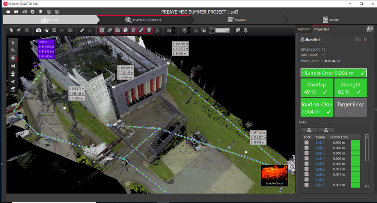
Figure 1: Coordinate extraction

STEP 4: Coordinate comparisons

The extracted coordinates of the truth solution (sol1 or sol1A) was compared to the other solutions (Sol2 to Sol10 or Sol 2A to Sol10A) to see how the changes in the ‘known’ target control point coordinates (errors) reflect on the model. The procedure adopted for the comparison was to copy the coordinates of the various solutions from the notepad files into excel spread sheet and then subtract the Easting, Northing and height(E,N,H) of the truth solution from the Easting, Northing and height of the other solutions (E,N,H) subsequently (see equations 1-3 and  figure 3.).

E2-E1=dE                                                                              [1]

N2-N1=dN                                                                             [2]

H2-H1=dH                                                                             [3]

Where:

E2, N2, H2 are the Easting, Northing and height of solution2.

E1, N1, H1 are the Easting, Northing and height of solution1.

dE= difference in Easting.

dN= difference in Northing.

dH= difference in height

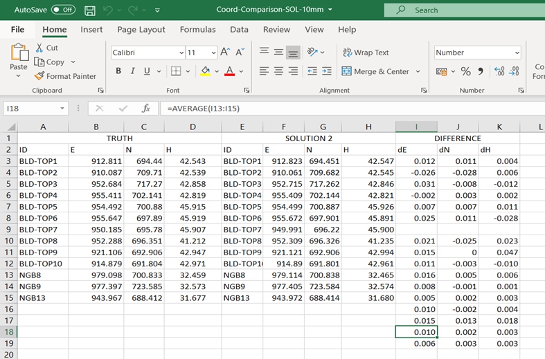
Figure 2: Coordinate comparison in excel spreadsheet

STEP 5: Coordinate transformation

To further understand the sensitivity of the model to the control coordinates adjustments (solutions), coordinate transformation was carried out as a second approach to substantiate the coordinate comparisons of the various solutions to the truth. Coordinate transformation is usually carried out from one reference frame to another. This is to show a quantitative and systematic shift of the model in the X, Y, Z axes from a reference frame 1 to a reference frame 2 with three translations Δx, Δy, Δz, three rotations Rx, Ry, Rz and a scale parameter μ as shown in equation 4. (Reit, 2010). In this project the reference frame 1 represents the coordinates of the truth-which is the three control targets and the eight corners of the building. While reference frame 2 represents the coordinates of Sol2-Sol10: which are the three targets and the eight corners of NGB. The Helmert estimation (transformation) spreadsheet was used to carry out the coordinate transformation between Sol1 and Sol2-Sol19 (figure 4).This was used because it is quite straightforward and uses least square solutions for the transformations. The Helmert estimation spreadsheet can solve for all seven parameters or at least three.

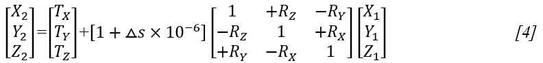
Where;

X_1, Y1, Z1 are the coordinates of the reference frame 1

X_2, Y2, Z2 are the coordinates of the reference frame 2

T_X, TY, TZ are translation along the X, Y and Z axes

R_X, RY, RZ are the rotations along the X, Y and Z axes and ⧍s is the scale.

Figure 3: Helmet transformation spreadsheet used for coordinate transformations

STEP 6: Volume comparison with LSS

The surface model of solution1 and solution 8-solution10 where further compared using LSS software. This comparison was done to further validate the coordinate comparison with respect to the adjustment of the truth coordinates affecting only the height components of the target controls. The area and volume of sol8-solution10 where then compared to the truth. The procedure involved include the following steps:

1. In Cyclone Register360 the registered model versions (Sol8-Sol10) where exported as .PTS file format.
2. Published report of the model solutions where then saved.
3. Each of the saved .PTS file was imported into LSS and convert to .LSS file format to produce e 3D model in LSS.
4. Terrain extraction using 3D vision in LSS was initiated to produce the surface models of the four solutions.
5. The area and volume of each solutions where then generated from LSS and the truth was then compared to the other three solutions, respectively (see figures 3a and 4a in appendix).

The steps taking for data import-target control point coordinates registrations, coordinate comparisons, and coordinate transformation in the first investigation were repeated for the second investigation. The registration with the six targets control points and data cleaning affects all the versions (solutions) once done.

RESULTS ANALYSIS AND DISCUSSIONS

Gerneral

The results of investigating the sensitivity of the Terrestrial Laser Scanning (TLS) model to the target control point coordinates of NGB10, NGB11 and NGB12 using the methodology described as presented in section 2.0, are outlined and discussed in this section as the results of the first investigation and the results of the repeated investigation.

First investigation – with 10mm in Easting and Northing and 20mm in height

The initial results of the first investigation, by adjusting the original control coordinates by 10mm to the easting and northing and 20mm to the height.

Data cleaning

As the NGB was the focus of the investigation, data cleaning was carried out to remove most of the surrounding features. This also helps in reducing the size of the huge point cloud to a much smaller amount in the bundle cloud as presented in (figures 5a and 6a in appendix) and figure 5.

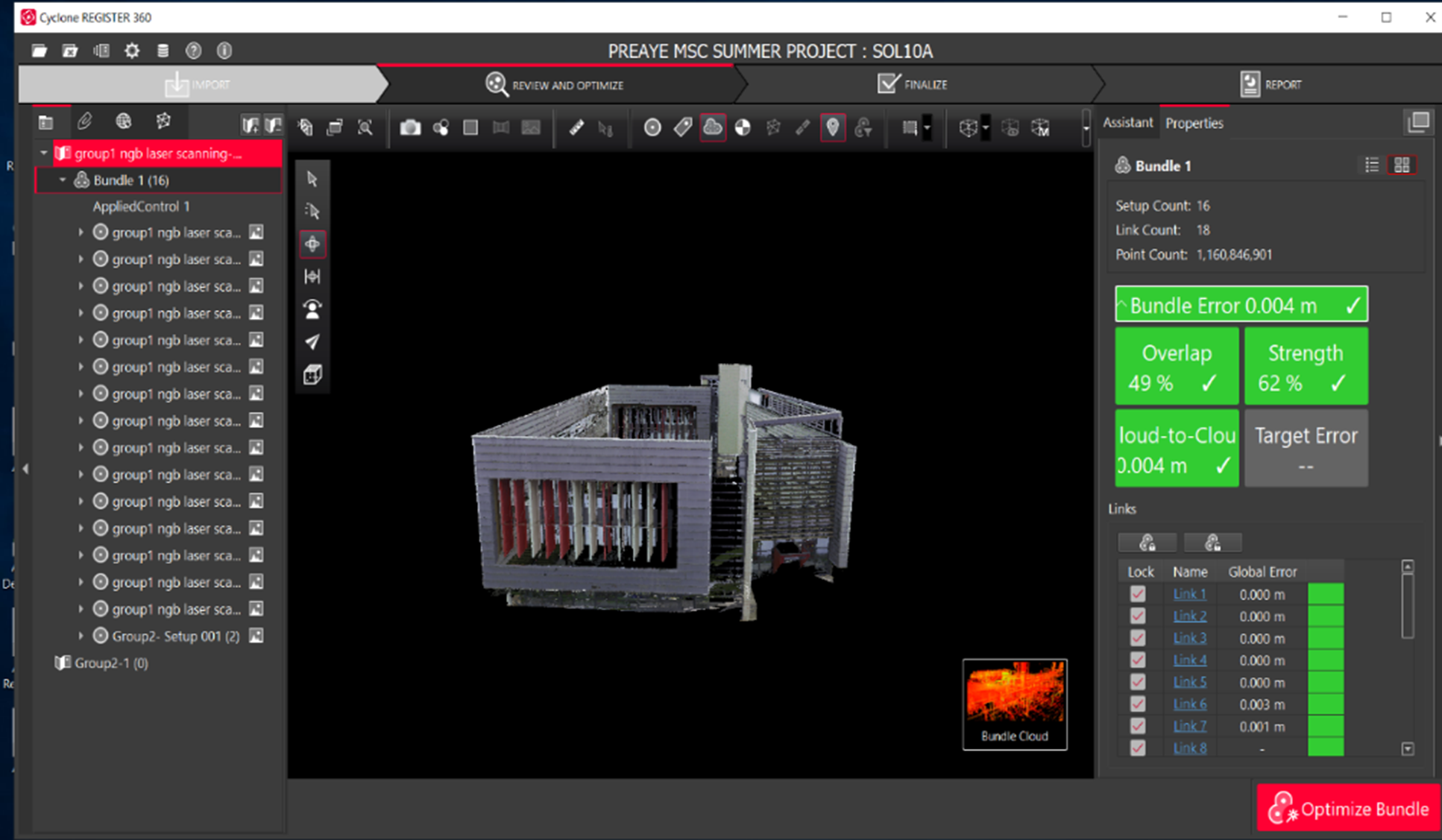
Figure 4: Improved version of bundle cloud of NGB after further cleaning

Registration with target control point coordinates (solutions)

The registration of the sixteen setups were carried out in the Cyclone software (figures 7a to 10a in appendix) showed the results of the registration for sol1, sol2 and sol3. In general, a red colour in the bundle statistics (Link Error, Strength and Cloud-to-Cloud error) indicates a weak bundle registration, while a green colour indicates a strong bundle registration. As seen in the statistics (figure 7a in appendix), the bundle registration was weak (strength of 23%) with a high value of cloud-to-cloud error of 0.027m amounting to a link error of 0.027m. This was caused by the misalignment of the point cloud during the registration process. In order to achieve a strong bundle registration, visual alignment was carried out to increase the strength to 59% and reduce the cloud-to-cloud error to 0.010m resulting to a lower link error of 0.010 m, as seen. The registration with different ‘known’ target control point coordinates for NGB10, NGB11 and NGB12 did not affect the quality of the bundle registration as shown in the statistics. This is because the coordinates are only used to transform the model from the local coordinate system to a global coordinate system. The same results were obtained for sol4 to sol10.See appendix.

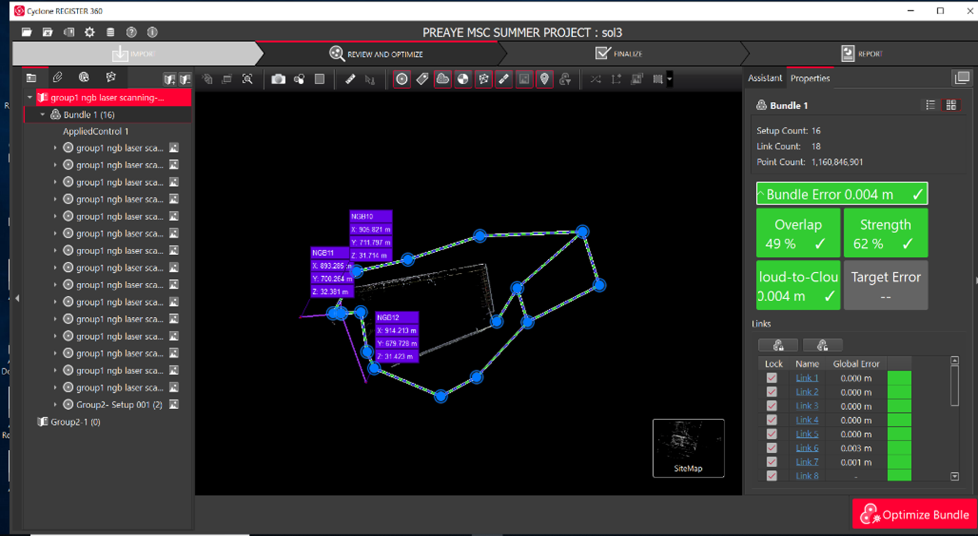
Figure 5: Bundle registration for sol3- with a 10mm difference in northing from the truth coordinates at NGB10, NGB11 and NGB12

Coordinate extraction

The coordinate extractions and comparisons were carried out in the same manner as in the previous section. Figures 7 show the results of the extracted coordinates of two of the top corners of NGB (BLD-TOP1 and BLD-TOP2) of sol1 and sol2 (figure 11a in appendix). Similar results were obtained for sol3 to sol10 .See appendix.

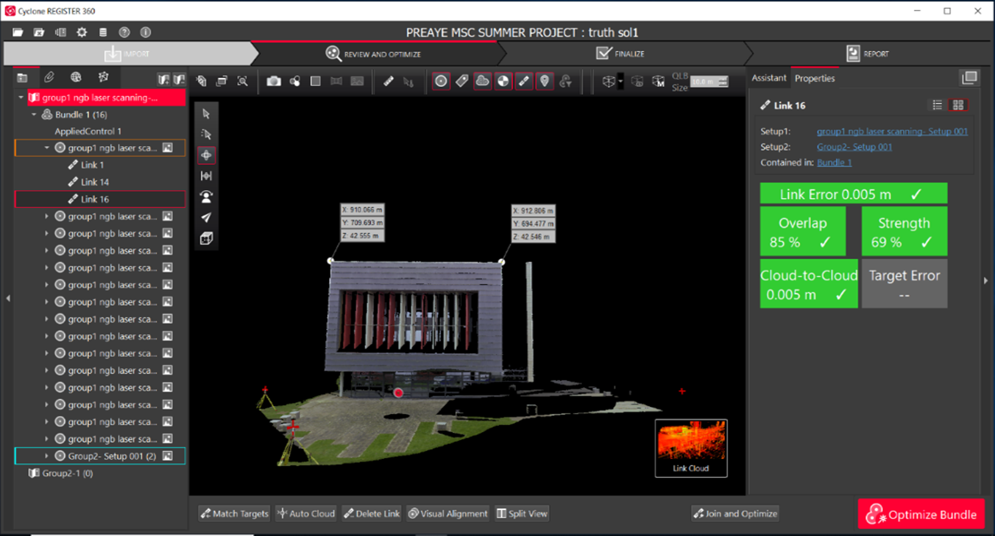
Figure 6: Coordinate extraction of building corner 1 and 2 from the model for sol1 -‘truth’

Coordinate comparison

The results of the final coordinate comparison for eight of the ten top corners of NGB (BLD-TOP1 to BLD-TOP6 inclusive, plus BLD-TOP8 and BLD-TOP9) and the three additional target control points (NGB8, NGB9 and NGB13) for sol2 to sol10 inclusive, with respect to sol1 – truth, are shown in figures 8.See also  figures 12a to 15a in appendix.

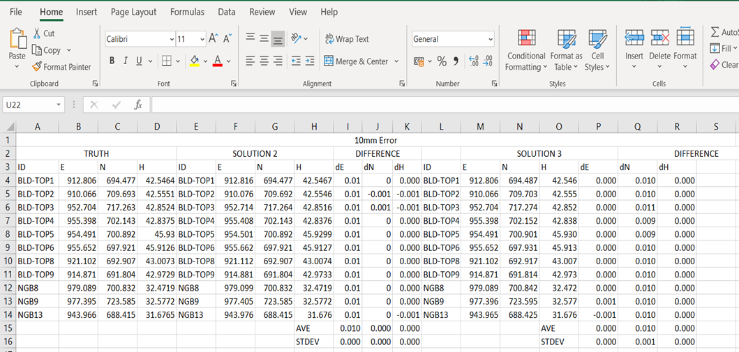
Figure 7: Excel spreadsheet results of coordinate comparison of sol2 and sol3 with sol1 – truth (sol2 – with a 10mm difference in easting from the truth coordinates at NGB10, NGB11 and NGB12; sol3- with a 10mm difference in northing from the truth coordinates at NGB10, NGB11 and NGB12)

The final results obtained from the coordinate comparison of sol1 (truth) and sol2 to sol10 inclusive shows more consistency in the amount of coordinate shifts from the truth, which reflect the added 10mm to the easting and northing and 20mm to the height in the various solutions. As seen in figure 35, the addition of 10mm to the easting or northing of all three ‘known’ target control points in sol2 and sol3 resulted in a corresponding systematic shift in the easting and northing of the eight top corners of NGB and the three additional target points. The results for sol4 to sol10 inclusive are summarised below:

1. The 10mm added to the Eastings of the coordinates of NGB10 and NGB11 in sol4 resulted in a rotation of the model in the easting direction. On average the points in the model moved by more than half of the original amount (10mm) added for the Eastings and less than half of that amount for the northings.
2. In sol5 the impact of the 10mm added to the northings of NGB10 and NGB11 is similar to that of sol4 but the rotation is in the north with a slight difference in the average amount of shift.
3. In sol6 and sol7, the 10mm added to the Easting and Northing separately at NGB10 caused movement of the different points by different amounts as seen in the coordinate comparison in figure thereby causing a positional shift of the model.
4. In sol8, the 20mm added to the height components of the ‘known’ target control point coordinates of NGB10, NGB11 and NGB12 caused a corresponding 20mm shift in the height dimension of the model and a slight shift in the Easting and Northing.
5. In sol9, the 20mm height adjustment to the ‘truth’ for NGB10 and NGB11 caused a varying amount of shift in the easting, northing and height in the model. While, in sol10, the 20mm added to the height component at NGB10 only also resulted in a positional shift in easting, northing and height.

From the analysis of the coordinate comparisons for sol2 to sol10 inclusive, it is evidently clear that the deformation in the positions of the ‘known’ target control points used in the scanning are transferred to the model in varying degrees.

Results with coordinate transformations

The results of the coordinate transformations of sol1 (truth) and sol2 and sol3 using the Helmert estimation spreadsheet with all seven parameters (delta x, delta y, delta z and theta x, theta y, theta z and scale) are presented in Figure 9. Similar results were obtained for sol4 to sol10 inclusive (see appendix).

Figure 8: Coordinate transformation with Helmert estimation spreadsheet using all seven parameters for sol 1 – truth and sol2 (sol2 – with a 10mm difference in easting from the truth coordinates at NGB10, NGB11 and NGB12)

The first sets of coordinate transformation results for sol2 and sol3 that were obtained from the Helmert estimation showed a large origin shift as well as large rotations, which were far more than the values added to the ‘known’ target control point coordinates .This large shift in origin/rotation is as a result of the least square equations trying to accommodate for the differences in the coordinates in the solutions and solve for all seven parameters(delta x, delta y, delta z, and theta x, theta y, theta z and a scale parameter).

A new approach was therefore conceived by considering that all seven parameters do not need to be solved for, as some of them are not relevant. In this approach, the almost North-South orientation of NGB10, NGB11 and NGB12 and the almost West-East orientation of the building were considered to decide which of the seven parameters were relevant in each case, as outlined below:

1. Solving for just four parameters (delta x, scale, theta x, theta y) for sol2, sol4 and sol6 on the assumption that a shift in Easting (x) at 2 or 1 of these points should cause a translation in Easting (delta x), a rotation in Easting and Northing (theta x, theta y) and possibly a change in scale( figure 10), but should not cause a translation in Northing and Height (delta y, delta z) or a rotation in Height (theta z).See figures  16a and 17a in appendix.

Figure 9 Coordinate transformation with Helmert estimation spreadsheet using four parameters for sol1 -truth and sol2 truth (sol2 – with a 10mm difference in easting from the truth coordinates at NGB10, NGB11 and NGB12)

2. Solving for only four parameters (delta y, scale, theta x, theta y) for sol3, sol5 and sol7 on the assumption that a shift in Northing (y) at 2 or 1 of these points should cause a translation in Northing (delta y), a rotation in Easting and Northing (theta x, theta y) and possibly a change in scale( figure 11), but should not cause a translation in Easting and Height (delta y, delta z) or a rotation in Height (theta z) as shown in in figures 18a and 19a in appendix.

Figure 10:  Coordinate transformation with Helmert estimation spreadsheet using four parameters sol1 – truth and sol3 (sol3 – with a 10mm difference in northing from the truth coordinates at NGB10, NGB11 and NGB12

3. Solving for only 3 parameters (delta z, scale, theta z) for sol8, sol9 and sol10 on the assumption that a shift in Height (z) at 2 or 1 of these points should cause a translation in Height (delta z), a rotation in Height (theta z) and possibly a change in scale, but should not cause a translation in Easting and Northing (delta x, delta y) or a rotation in Easting and Northing (theta x, theta y) as seen in figures 12. See also figures 21 and 22 in appendix.

Figure 11: Coordinate transformation with Helmert estimation spreadsheet using three parameters for sol1 – truth and sol8 (sol8 – with a 20mm difference in height from the truth coordinates at NGB10, NGB11 and NGB12)

The results obtained with the Helmert estimation spreadsheets for the coordinate transformations of sol1 (truth) and sol2 to sol10 inclusive with less parameters, clearly showed more systematic shifts of the model that are consistent with the results derived in the coordinate comparisons with the Excel spreadsheet, and reflect the various combination of an added 10mm to the Easting and Northing and 20mm to the height in sol2 to sol10 inclusive. The analysis of the coordinate transformations of sol2 to sol10 inclusive shows that the deformation in the positions of the ‘known’ target control points are replicated into the model in the form of translations and/or rotations to the top corners of NGB and the additional target control points.

Results of volume comparisons with LSS

Although the above results are quite conclusive, it is often the practice when using laser scanning to not compare individual points but to compare two digital surface models, in order to quantify any deformation as a change in volume. A volume comparison was, therefore, undertaken using LSS software to further understand the impact of the 20mm added to the ‘known’ target control point height components at NGB10, NGB11 and NGB12 on the resultant digital surface models. The results of the surface models and the reports of the area and volume computations for sol8, sol9 and sol10 in comparison to sol1 (truth) are shown (see figures 23a- to 32a inclusive in appendix.

A summary of the area and volume comparison reports from LSS is presented in Table 4.1 below:

Table 4. Summary of area and volume comparison reports of digital surface modes (sol1-truth with, sol9 and sol10) from LSS

Surface description	Cut area (m2)	Cut volume(m3)	Fill area(m2)	Fill volume(m3)	Total area(m2)	Net volume(m3)
Sol1&Sol8	961.167	-21.837	11.136	2.124	972.305	-19.714
Sol1&Sol9	652.040	-40.068	319.830	39.493	971.870	-0.575
Sol1&Sol10	858.596	-71.471	113.183	43.661	971.779	-27.809

From an analysis of the area and volume comparison reports, the following observations can be made:

1. The comparison of the digital surface models of sol1 – truth and sol8 shows that by adding 20mm to the height components of all of the ‘known’ target control points (NGB10, NGB11 and NGB12) resulted in a deformation with net volume of -19.714m³.
2. The comparison of the digital surface models of sol1 – truth and sol9 shows that by adding 20mm to the height components of two of the ‘known’ target control points (NGB10 and NGB11 and not NGB12) resulted in a deformation of the model by a net volume of almost zero (-0.575m³) as sol9 is effectively tilted along a central axis with respect to sol1.
3. The comparison of the digital surface models of sol1 and sol10 shows that by adding 20mm to the height component of only one of the ‘known’ target control points (NGB10 and not NGB11 or NGB12) resulted in a deformation of the model by the largest net volume (-809m³) suggesting that sol10 is also tilted with respect to sol1 but not along a central axis.

These results are consistent with the fact that there are rotations apparent in the coordinate transformations for sol9 and sol10 which then lead to the above tilts, but what is clearly interesting is how such tilts from relatively small adjustments in the height component of the ‘known’ target control points can lead to massive apparent changes in volume.

Final results of the repeated investigation – with 100mm in Easting, Northing and height

The final results of the repeated investigation with- 100mm in Easting, Northing and height for the registration, coordinate extraction and comparisons as well as transformations for the truth and sol2-sol10 are presented in the section. The procedures for obtaining these results remain the same as in the initial results with the 10mm and 20mm solutions. These later results not only further substantiated the results of the former, but also captures the magnitude of the 100mm adjustments to the truth .See appendix.

CONCLUSION

Monitoring for quantifiable and geometric changes in objects with terrestrial laser scanner is often assumed to be caused by environmental factors such as long use, rise in ground water level, heat, etc.

Analysis of the results of the coordinate comparisons of eight top corners of the building NGB (BLD-TOP1 to BLD-TOP8) and the three target points of the different solutions (sol1-sol10) of the model shows difference in coordinates of the same points in the different models corresponding to the amount of deformations introduced (10mm and 20mm for the first investigation and 100mm for the second investigation). Again, the analysis of the results in the coordinate transformations with Helmert estimation of the different solutions (so1-sol10) of the top corners of the building (BLD-TOP1 to BLD-TOP8) and the three target points reveals systematic shifts in the form of translation/rotation of the model in agreement with the coordinate comparisons. Furthermore, the volume comparisons of different surface models (sol8-sol10) to the truth-the original surface model-shows how a little deformation in the height of the target control point coordinate will translate to a massive volume difference in the models as compared to the original surface model. These apparent changes in the geometry of the model is clearly induced by the deformations of the target control points used-the subtle changes to the control coordinates (truth).

This research findings have demonstrated the impact of the two possible scenarios earlier stated on the TLS model and thereby fulfilling the aim and objectives outlined. The sensitivity of TLS model to target control point coordinates that has been revealed in this investigation has shown that the use of volume comparison  in TLS model in deformation monitoring can be misleading especially when the changes in volume is attributed to other factors. The volume changes in the monitored object as seen in the NGB model was influenced by deformation of the target control points used in the registration process of the raw point cloud.  The subtle changes in the target control points can significantly affect the accuracy of the model. This research has practically demonstrated the fact that TLS model is sensitive to the target control points in deformation monitoring. Errors in the target control point coordinates can cause deformation (volume changes) in the model.

In other to reduce or eliminate the effect of coordinate errors in the model, the controls used in deformation monitoring should be well established with high level geodetic instruments such as differential GPS and total station. Also, the controls to be used for deformation monitoring that has been established prior to monitoring with TLS should be confirmed to be in their right positions.

It is recommended that the investigation be repeated with using known target heights of the three target points of NGB8, NGB9 and NGB13 to understand how the combinations of the six target height control points would affect the model. Also, the laser scanning of NGB should be repeated at different periods with same solutions for the processing. Furthermore, the investigation should be repeated with other features for comparison.

ACKNOWLEDGEMENT

The author wish to acknowledge the support of the Petroleum Technology Development Fund (PTDF) in the award of scholarship to study a post graduate degree in the University of Nottingham, United Kingdom that led to this research work. Special thanks also to Prof Richard Bingley, for his guidance and mentorship during the execution of this research work.

REFERENCES

1. Lindenbergh, R. 2013. Trends in detecting changes from repeated laser scanning data:  Proceedings of the Joint International Symposia on Deformation Monitoring, Nottingham, United Kingdom, September 9-10.
2. Abbas, M A., Fuad, N A.., Idris, K M. and Sulaiman, S A^. 2019. Reliability of Terrestrial Laser Scanner Measurement in Slope Monitoring. Earth and Environmental Sciences, Volume 385,4^th International Conference on Research Methodology for Build Environment and Engineering Chulalongkorn University, Malaysia, 24- 25 April.
3. Barber, D.; Mills, J.; Smith-Voysey, S. 2008. Geometric validation of a ground-based mobile laser scanning system. ISPRS J. Photogramm. Remote Sens., 63, 128–141.
4. Erol, S., Erol, B, and Ayan, T. 2004.  A general review of the deformation monitoring techniques and a case study: analysing deformations using GPS/levelling. International Archives of Photogrammetry, Remote Sensing and Spatial Information Sciences, 35(B7), pp.622-627.
5. Paweł B. Dąbek, Ciechosław Patrzałek, Bartłomiej Ćmielewski & Romuald Żmuda. 2018. The use of terrestrial laser scanning in monitoring and analyses of erosion phenomena in natural and anthropogenically transformed areas, Cogent Geoscience, 4:1, 1437684.
6. Asteris, P. G and Plevris, V.2015.Handbook of Research on Seismic Assessment and Rehabilitation of Historic Structures-26.1 Introduction, pp. 754. Retrieved from http://app.knovel.com/hotlink/pdf/id:ktOOURMJNF/handbook-research-seismic/laser-scan-introduction (11th March, 2020).
7. Wujanz, D., Krueger, D. and Neitzel, F. 2013. Defo scan++: surface-based registration of terrestrial laser scans for deformation monitoring. In: Proceedings of the Joint International Symposia on Deformation Monitoring, Nottingham, United Kingdom, 910 September.
8. Litchi, D.D. and Gordon, S.J.2004.Error propagation in directly georeferenced terrestrial laser scanner point clouds for cultural heritage recording. Proceedings of FIG Working Week, Athens, Greece, May 22-27.
9. Charalambous, E., Psimoulis, P., Guillaume, S., Spiridonakos, M., Klis, R., Bürki, B., Rothacher, M., Chatzi, E., Luchsinger, R., Feltrin, G. (2015), Measuring sub-mm structural displacements using QDeadalus: a Conference on Computing in Civil and Building Engineering (ICCCBE), Nottingham, UK, 30 June-2 July.
10. Abbas, M. A., Setan, H., Majid, Z., Chong, A. K., Lichti, D. D., Idris, K. M. and Ariff, M. F. M. (2013) Self-calibration for accuracy enhancement of hybrid and panoramic scanners. Proceedings of the Joint International Symposium on Deformation Monitoring, Nottingham, United Kingdom, September 9-10.
11. Alba, M., Fregonese, L., Prandi, F., Scaioni, M. and Valgoi, P. 2006. Structural monitoring of a large dam by terrestrial laser scanning. International Archives of Photogrammetry, Remote Sensing and Spatial Information Science, 36(5), pp. 6, (on CD-ROM).
12. Borne, Leandro. Lingua, Andrea. and Rinaudo, Fulvio. 2002. Engineering and environmental applications of laser scanner techniques. International Archives of Photogrammetry, Remote Sensing and Spatial Information Sciences, 34, pp. 40-43.
13. Dunnicliff, J. 1993.In: Geotechnical instrumentation for monitoring field performance. New York, Wiley.
14. Fröhlich, C and Mettenleiter, M.2014. TERRESTRIAL LASER SCANNING – New Perspectives in 3D Surveying International Archives of Photogrammetry, Remote Sensing and Spatial Information Sciences Vol xxxvi 8/W2.
15. Grimm, D and Zogg, H.-M. 2008. Dynamic Monitoring of Load Tests by Kinematic Terrestrial Laser Scanning. Proceedings of 6^th Swiss Geoscience Meeting, Lugano.
16. Han, J., Guo, J. and Jiang, Y. 2013. Monitoring tunnel profile by means of multi-epoch dispersed 3-D LIDAR point clouds. Tunnelling and Underground Space Technology, 33, pp.186-192.
17. Lemmens, M. 2011. Terrestrial Laser Scanning. Geo-information. Geotechnologies and the Environment, vol5. Springer, Dordrecht
18. Li, J., Wan, Y. and Gao, X. 2012. A new approach for subway tunnel deformation monitoring: high-resolution terrestrial laser scanning. International Archives of Photogrammetry, Remote Sensing and Spatial Information Sciences, 39(B5), pp. 223-228.
19. Lindenbergh, R., Uchanski, L., Bucksch, A. and van Gosliga, R. 2009. Structural monitoring of tunnels using terrestrial laser scanning. Reports on Geodesy, 2(87), pp. 231–239.
20. Litchi, D. D., Gordon, S. J. and Stewart, M. P. 2002a. Ground-based laser scanners: operations, systems and applications. Geomatica, 56(1), pp.21-33.
21. Mills, J. and Barber, D. 2014. Geomatics Techniques for Structural Surveying. Journal of Surveying Engineering 130 (2), 56-64.
22. Moodle lecture material, 2020.Deformation surveying and practical, University of Nottingham UK.
23. Mukupa, W., Roberts, G. W., Hancock, C. M. and Al-Manasir, K. 2016a. A review of the use of terrestrial laser scanning application for change detection and deformation monitoring of structures. Survey Review, pp. 1-18.
24. Mukupa, W. 2017. Change detection and deformation monitoring of concrete structures using terrestrial laser scanning. Unpublished PhD thesis, Department of Civil Engineering, University of Nottingham UK.
25. Panagiotis G and Plevris, Vagelis. (2015). Handbook of Research on Seismic Assessment and Rehabilitation of Historic Structures – 26.1 Introduction. (pp. 754). IGI Global. Retrieved from https://app.knovel.com/hotlink/pdf/id:kt00URMJNF/handbook-research-seismic/laser-scan-introduction (2 Feb 2020).
26. Psimoulis, P., and Stiros, S. (2007), Measurement of deflections and of oscillation frequencies of engineering structures using Robotic Theodolites (RTS). Engineering Structures, 29(12), pp. 3312-3324.
27. Schäfer, T., Weber, T., Kyrinovič, P. and Zámečniková, M. 2004. Deformation measurement using terrestrial laser scanning at the hydropower station of Gabcikovo. In: Proceedings of INGEO 2004 & FIG Regional Central & Eastern European Conference – Engineering Surveying, Bratislava, Slovakia, and 11-13 November.
28. Shan, J. and Toth, C. K eds.2009.Topographic Laser Ranging and Scanning: Principles and process. Boca Raton, CRC press.
29. Shan, J. and Toth, C.K.2918. Topographic Ranging and Scanning: Principles and processing.2^nd edition. London Press.
30. Stagier, R 2003.Terrestrial laser scanning- technology, systems and applications. Proceedings of 2^nd FIG Regional Conference, Marrakech, Morocco, December 2-5.
31. Stiros, S., Psimoulis. P., Kokkinou, E. (2008). Errors introduced by fluctuations in the sampling rate of automatically recording instruments: Experimental and theoretical approach. Surveying Engineering, 134(3), pp.89-93.
32. Vosselman, G. and Maas, H.G. 2010. Airborne and terrestrial laser scanning. Dunbeath: Whittles Publishing.
33. Wang, J.2013.Block to fine registration in terrestrial laser scanning. Remote Sensing, 5, pp. 6921-6937.