
“Effect of Economic Growth on the Environment in Bangladesh”
- Md Kamrul Islam
- Khawaja Saifur Rahman
- Saiyara Fairooz
- 830-845
- May 10, 2023
- Environment
“Effect of Economic Growth on the Environment in Bangladesh”
Md Kamrul Islam, Khawaja Saifur Rahman, Saiyara Fairooz
Economics, Indepenedent University Bangladesh
DOI: https://doi.org/10.47772/IJRISS.2023.7469
Received: 27 March 2023; Revised: 09 April 2023; Accepted: 12 April 2023; Published: 10 May 2023
ABSTRACT
The objective of the study is a practical investigation of the Environmental Kuznets Curve (EKC) hypothesis in the case of Bangladesh.
Data used is from 1986 to 2014. Data has been collected from the official world bank databank website. The autoregressive distributed lag (ARDL) approach will be used for the short-run analysis and a vector error correction model (VECM),a bounds test for cointegration will be used to find the long-run relationships. We will be examining the dynamics between economic growth, foreign direct investment, and energy consumption with carbon dioxide emissions in Bangladesh.
We find that income has a very modest negative effect on the environment and pollution in the long run. Energy consumption is discovered to be a bigger contributor to carbon dioxide emissions in the country, especially in the short run.
In the case of FDI inflow, the relationship is found to be negative with environmental degradation, but in the long ,haul the value does gravitate towards a positive link, however negligible.
INTRODUCTION
Over many years research is ongoing on how economic growth may or may not have impacts on the environment. Primarily, the researchers tried to find whether the Environmental Kuznets curve exists in real life. It is an upside down U shaped curve plotted on a graph with per capita income growth on the y-axis representing economic growth and environmental quality on the x-axis.
Now with major and pressing issues worldwide such as global warming and climate change, finding the relationship between economic growth and nature’s deterioration is becoming more and more crucial.
Major sources say that carbon dioxide emissions through combustion of fossil fuels is the most significant contributor to global warming. This took researchers attention to work on finding a relationship between energy consumption and quality of the environment.
Recent discoveries under the literature of this issue reveal that pollution intensive industries are shifting towards being more concentrated in developing countries since developed countries are switching towards stricter environmental laws and regulations due to existence of trade treaties (e.g WTO treaties). Therefore, including a relevant variable such as FDI when examining the relationship between growth and environmental deterioration will help empirical evidence in the literature of this topic. It will also help us to find out whether developed economies shift pollution-intensive production to less developed nations (such as Bangladesh), and operate cleaner production techniques in their own economies.
Incorporating energy consumption as a variable is also important to see what effect it has on the environment quality besides income growth. A lot of research has been done in the past to find the existence of the Pollution Haven Hypothesis (PHH) which suggests that polluting industries tend to relocate or set up in areas with a laxer law and jurisdiction. These industries cannot be set up in the developed areas due to the stringent environmental laws and regulations. Most studies have found the existence of this behavior. If a host country lacks strict environmental laws, inflow of FDI mostly results in pollution and degradation of environmental quality. The aim of this study is to contribute to existing literature on this topic by finding the relationship between growth and environment in one developing country; Bangladesh while controlling for both energy consumption and FDI. We will be using the ARDL ECM method to estimate the parameters.
We will attempt to find out whether there is a Kuznets curve for Bangladesh over this time period or not, by analysing the direct relationship between income growth and environmental state.
LITERATURE REVIEW
Current knowledge on this topic shows that there in fact is a relationship between economic growth and nature’s quality. In developing countries, development and environment degradation are mostly seen to be positively correlated whereas in developed countries there is a negative relationship. This also proves that the EKC (Environmental Kuznets Curve) theory holds in real life.
Various studies on different countries or multiple countries have provided evidence for the fact that the link between ecological quality and income per head exhibits a variety of patterns; in some cases the relationship is found to be positive, and negative in others. (Shafik, 1994).
Kim, Hyun & Baek, Jungho. (2011) found negative relationship amid income and co2 emission in the developed economies, positive relationship in developing economies providing empirical evidence for EKC curve. They’ve used the ARDL error correction model and incorporated energy consumption and FDI into the model to find the existence of EKC in 40 countries with data covering 1971 to 2005. The results show positive correlation among energy consumption and carbon di-oxide emission for most countries in the long run and the relationship between FDI and co2 emission are concluded as not significant. However, in the short run increasing income and energy consumption are found to be the major contributors to pollution.
Jungho Baek and Won W Koo have used the ARDL approach and found a positive correlation between GDP and CO2 production is both India and China in their paper “A Dynamic Approach to the FDI-Environment Nexus: The case of China and India ”. They further came across strong short run and long run positive correlation allying FDI and CO2 emission in China. In India FDI inflow is found to exacerbate the nature quality in the short run, but has negligible impact in the big picture or in the long run.
Shafik et al. (1994) have theorised the role that globalisation has on the growth and natural degradation nexus. He talks about how having an open trading regime leads to higher employment of a more clean production procedure; liberalization and improved competency will lead to investment expansion in technology and eventually encourage adapting to cleaner productive methods, thereby helping to meet higher environmental standards.
On the other hand, Angelsen and Kaimowitz (1999) concluded that development and liberalization of economies both can possibly intensify deforestation in “Rethinking the Causes of Deforestation: Lessons from Economic Models”. Intrusion in agriculture, commercial use of wood and deforestation all seem to be interrelated and required for development and growth.
Likewise, in the report of Neumayer (2000) trade, liberalization, development and growth, are promoted by globalisation, forsaking natural resources and sustainability.
Watson et al. (1998) insists that various aspects such as the greenhouse effect, climate change etc, are global in scale. These are consequences of countless previous economic transactions and actions that were considered to be crucial for development. Thus, a comprehensive and international effort and co-ordinated control system is vital now, though laborious to achieve since nothing of this sort has been attained as of yet.
Muah et Al., (2010) established a straight line relationship amid income per head and co2 release in most cases in Bangladesh.
Amin, Ferdaus and Porna (2012) used data from 1976 to 2007 and a multivariate vector error correction model for analysing the link between co2 discharge, output and energy use in Bangladesh in “Causal Relationship among Energy Use, Co2 Emissions and Economic Growth in Bangladesh: An Empirical Study”. They find no relationship between output and amount of co2 released in the short run, however energy use is concluded to be a major cause of co2 emissions.
Janifar Alam found a positive connection between quantity of co2 emitted and per capita GDP of Bangladesh from 1972 to 2010, but no signs of fall in pollution yet, thus concluded to find no existence of EKC curve.
Or we can infer from this result that even if there is a potential Kuznets curve for Bangladesh, the country has not yet reached or surpassed peak pollution point to proceed to becoming a developed country. So, the whole curve does not exist for the country as of 2010. She has used data of CO2 emission in per capita metric tons and per capita GDP in current $US from 1972 to 2010.
Jungho Baek and Yoon Jung Choi find in their paper “Does Foreign Direct Investment Harm the Environment in Developing Countries? Dynamic Panel Analysis of Latin American Countries”
They have used data of 41 years, from 1971 to 2011 of panel data of 17 Latin American countries and used ARDL as methodology.
In “Energy consumption, carbon emissions and economic growth nexus in Bangladesh: Cointegration and dynamic causality analysis” Jahangir Alam, M., Ara Begum, I., Buysse, J. and Van Huylenbroeck, G2012, they used data from 1972 to 2006 of per capita real GDP for economic growth, energy consumption per capita (in kg of oil equivalent), electricity consumption (kiloWatts per hour) and co2 emission (in metric tonnes) to measure pollution in environment. They used ARDL ECM model for
Holtz-Eakin and Selden (1995) discovered a monotonous rising EKC curve whereas Friedl and Getzner (2003) came across a sort of n-shaped curve.
“Under an optimistic perspective the EKC might be taken to suggest that economic growth is not a threat to global sustainability, and there are no environmental limits to growth” (Stern et al., 1996).
In contrast, Arrow et al., (1996) came to the conclusion that development is not an elixir or cure to the environmental issues; sustainable development ideally has the ability to control economic, social and environmental issues, and overseeing any one of these can jeopardize the overall economic progress.
From this perspective, globalisation may give the impression that environmental improvement will be achieved more easily with more integration, only to actually provide the last push that should help to cross the EKC turning point.
In “Environmental Kuznets Curve: the case of Bangladesh for waste emission and suspended particulate matter” by Md Danesh Miah, Md Farhad Hossain Masum, Masao Koike, Shalina Akther and Nur Muhammed, they have found short run evidence of EKC trend in Bangladesh, where environmental degradation is positively related to income growth, using SPM as an indicator for environmental degradation.
Chandra Ghosh, (2014) found that energy use increases with economic expansion, while link among economic growth and carbon emissions relationship is not statistically significant in Bangladesh.
Jungho& Won W., (2009) have assessed the relationship between GDP, FDI and co2 emissions in China and India in their paper “A Dynamic Approach to the FDI-Environment Nexus: The Case of China and India”. They find a positive correlation between FDI and co2 emissions in China in both the short and long run. However, in India FDI affects co2 emissions negatively in the short run and has insignificant outcomes for the long run. In case of GDP, co2 emissions increases with GDP in both the countries.
This portion of the literature review will examine the various measures that the government has taken to mitigate environmental damage caused by economic development.
The Bangladesh government has implemented various environmental laws and regulations, such as the Environmental Conservation Rules, the Bangladesh Environment Conservation Act, and the Bangladesh Environment Court Act. These laws and regulations are designed to protect the environment and promote sustainable development.
One of the most significant policies implemented by the government of Bangladesh to reduce the effect of economic growth on the environment is the National Environment Policy (NEP) of 1992 and revised in 2002.The policy provides a framework for sustainable development and includes measures to protect the environment, including reducing pollution and promoting renewable energy sources. The policy emphasizes the need for environmental impact assessments (EIAs) for all development projects and provides guidelines for conducting EIAs.
Another crucial policy implemented by the government of Bangladesh is the Environmental Conservation Rules of 1997. These rules require industries to obtain environmental clearance certificates before starting operations. The rules also provide guidelines for waste management and the disposal of hazardous waste.
The Forest Act of 1927 has also been revised to strengthen the protection of forests and promote afforestation.
The government of the country even implemented the Climate Change Strategy & Action Plan of 2009. This plan discusses the strategies in plan for adapting to and removing the negative effects of climate change such as mitigating greenhouse gas emissions, improving energy efficiency, and using more renewable energy.
In addition to these policies, the government of Bangladesh has implemented the Bangladesh Climate Change Trust Fund (BCCTF) to finance climate change adaptation and mitigation projects. The fund is managed by the Ministry of Environment, Forest and Climate Change and has financed various projects, including the construction of cyclone shelters and the implementation of renewable energy projects.
Sustainable, resilient and healthy environment; is one of the five Strategic Priority Areas for involvement of UNSDCF (The United Nations Sustainable Development Cooperation Framework) 2022-2026.
The government of BD has also implemented multiple initiatives for promotion of renewable energy sources. In 2010, the government launched the Renewable Energy Policy to promote the use of renewable energy sources such as solar, wind, and biomass. The policy aims to increase the share of renewable energy in the country’s energy mix to 10% by 2020 and 20% by 2030.
The government has also implemented several projects aimed at promoting renewable energy. The Solar Home System Project, for example, provides solar panels to households in rural areas to replace kerosene lamps and reduce indoor air pollution. The Rural Electrification and Renewable Energy Development Project aims to provide electricity to rural areas through the use of renewable energy sources.
The government of Bangladesh has also taken measures to improve waste management. The Solid Waste Management Act of 2010 provides a legal framework for the management of solid waste and promotes the use of recycling and composting. The government has also implemented several projects aimed at improving waste management, including the Municipal Services Project, which aims to improve waste collection and disposal in urban areas.
The government of Bangladesh has implemented a range of policies and initiatives aimed at reducing the adverse effects of economic growth on the environment. These measures include policies to protect the environment, promote renewable energy sources, and improve waste management. While much remains to be done to address the environmental challenges facing Bangladesh, these initiatives are an important step towards achieving sustainable development.
There has not been nearly enough study on Co2 emission, economic growth and quantity of energy used in Bangladesh. The proposed study intends to bridge these gaps and also include the effect of FDI along with these.
Theoretical Framework
The theoretical framework for this research paper is based on the Environmental Kuznet hypothesis that was initially proposed by Simon Kuznets in the late 20th century.
EKC hypothesis and background:
Simon Kuznets is the economist who first proposed a hypothesis linking the gini coefficient with economic growth. He’s a Russian- American economist who observed that as economic growth rises, income inequality will also rise but in the long run it will eventually disappear. This link is depicted by a reversed U shaped curve which is named “Kuznets Curve”.
In 1991 Grossman and Krueger linked the Kuznets curve with the environment in their study with NAFTA (Grossman and Krueger 1991; Stern 2004; Bhat-tarai and Hammig 2001). A curve illustrating the reversed U shaped relationship between environmental degradation and income per capita. In 1994 this was named Environmental Kuznets Curve (EKC) (Selden and Song 1994). It says that the environment degrades in the first stages of development with increasing income, however the deterioration diminishes later in the long run with rising income. (figure shown below)
The trouble with the kuznets curve is the assumption that income growth causes lies with the assumption of a causal role of income growth and the inadequacy of reduced-form specifications that presume that a common income-related process, conditional on fixed effects for political jurisdictions and a few observable covariates, adequately describes the generation of the pollutant of interest” (Carson 2010:5). In general, the effect dominates in the fast growing and the middle-income economies. So, increases in pollution and other degradation tend to overwhelm the time effect. In developed economies, growth rate is slower; and pollution reduction efforts can overcome the scale effect. This argument provides a foundation for the origin of the so- called EKC effect. Many developing countries are now addressing and even trying to remedy the pollution problems (Dasgupta, Laplante, Wang and Wheeler 2002)
The deterioration in the environment initially may seem sharper than the reduction portion later.
Income per capita is on the X axis and in the Y axis is the degradation of the environment.
A hill-shaped Environmental Kuznets curve is depicted below:
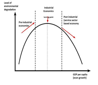
As we can see, the level of environmental degradation reaches its peak as economic growth takes place in an economy or country. As the economy continues to grow, environmental degradation declines again after a certain point, after which producers and consumers are both more aware of the environmental effects.
In the initial phase of development (pre-industrial economies), an economy focuses more on growing than on saving the environment or looking at the negative spillover effects of economic growth. The Kuznet curve tries to explain how in the beginning, a country would typically shift to mechanization in the agricultural sector and experience industrialization and the cities begin to attract people and labor from everywhere. Agriculture workers or farmers prefer to migrate to the cities for jobs, housing, better opportunities, education, healthcare, etc. This is the phase where the economy is growing at the fastest pace and environmental effects start to rise.
After a certain point income per capita increases, technology improves, solar and renewable energy are accessible to developed economies, environmental regulations become stricter, citizens become more aware and focus on living standards instead of real GDP as a measure of development. All these lead to greater environmental awareness and reduce environmental degradation. Industries have to follow a more stringent environmental screening process, where minimal pollution is allowed for the industry to operate. Through development, an economy also typically goes through a structural change where the economy shifts to being more service based than manufacturing or agriculture.
The Model
To analyse the consequences growth has on the environment, we will be using a theoretical framework that was put in place by Baek et al. (2009)
lnCt =β0+β1lnYt +β2lnEt+β3lnFt+εt
where,
C = Carbon Dioxide Emission (metric tons per capita)
Y = adjusted net national income per capita (current $US)
E = Energy consumption (measured in kg of oil equivalent per capita)
F= Foreign direct investment, net inflows (BoP, current $US)
εt= Error term.
Here, Ct is the pollution indicator we are using for this paper. This is our dependent variable. εt is the error term. The data has been collected from World development indicators, Worldbank database.
We want to find out whether there is a Kuznets curve for Bangladesh. For that we need to investigate both the short and long run relationships that income growth and co2 emissions portray.
Hypothesis:
H0 (null hypothesis): there is no link between rise in income and carbon emissions
H1(alternate hypothesis) : H0 is not true
DATA ANALYSIS
As we are working with time series data, there are chances of spurious regression results due to non-linearity. To solve this problem, we have taken the log values of all the variables and got rid of non-linearity. However, we have to also make sure all variables being used are stationary and are integrated of the same order.
The variables at level are non-stationary even in their log forms, found via ADF, Augmented dickey fuller test. It is a test used to reject or accept the null hypothesis that a unit root exists in the time series.
H0= Unit root exists
H1= H0 is not true
The augmented dickey fuller specifies the number of lags unlike the dicky fuller test, that is the only difference. In my analysis, I have generated new variables with 1 lag and used those variables for the tests.
We’ve used stata 13 for this test.
The null hypothesis (H0) here is that the variable has a unit root.
The alternate hypothesis says that the variable is generated stationarily.
The variables have been converted to log in the dataset. Newly lagged variables have also been generated after testing for optimal lag. We have found 1 to be the optimal lag for all the variables here. The Dickey fuller tests are run using the lagged variables at level.
None of the variables here are stationary at level. P values are above 0.05 and absolute value of test statistic is lower than all critical values. As a result, we cannot reject the null hypothesis and at level these variables are concluded to have a unit root or are non-stationary.
The results from the Dickey fuller test for unit root test or stationarity at first difference for all the lagged variables generated is shown here:
(Number of observations: 27)
| Dfuller co2 emission | Test statistic | 1% Critical value | 5% Critical Value | 10% Critical value |
| Z(t) | -6.462 | -3.736 | -2.994 | -2.628 |
| MacKinnon p-value for Z(t) | 0.0000 |
(Number of observations: 27)
| Dfuller income | Test statistic | 1% Critical value | 5% Critical Value | 10% Critical value |
| Z(t) | -3.191 | -3.736 | -2.994 | -2.628 |
| MacKinnon p-value for Z(t) | 0.0205 |
(Number of observations: 27)
| Dfuller energy use | Test statistic | 1% Critical value | 5% Critical Value | 10% Critical value |
| Z(t) | -7.435 | -3.736 | -2.994 | -2.628 |
| MacKinnon p-value for Z(t) | 0.0000 |
(Number of observations: 27)
| Dfuller FDI | Test statistic | 1% Critical value | 5% Critical Value | 10% Critical value |
| Z(t) | -6.011 | -3.736 | -2.994 | -2.628 |
| MacKinnon p-value for Z(t) | 0.0000 |
The p-values of all variables in the tests here are much less than 0.05. The test statistics are all significant and much less than the 1% critical value(except that of income, which is significant at 5% critical value).
The test statistics all being significant and p-values from these outcomes, tell us that the variables are all stationary at first difference. We can reject the null hypothesis that says unit root exists and conclude data to be stationary.
After that we run a test to check whether the series has heteroskedasticity. Heteroskedasticity means there are more dispersions in some data compared to the others. Variance of some variables or one variable is different, and not parallel to that of other variables.
The result is shown below.
| Heteroskedasticity Test: Breusch-Pagan-Godfrey
Null Hypothesis: Homoscedasticity |
|||
| F stat | 0.425208 | Prob. F(14,10) | 0.9300 |
| Obs* R-squared | 9.328874 | Prob. Chi-Square(14) | 0.8094 |
| Scaled explained SS | 1.128284 | Prob. Chi-Square(14) | 1.0000 |
As the results depict, a prob. Chi square value of 0.8094 is higher than 0.05. Thus we cannot reject the null hypothesis.
We accept the null hypothesis of Homoscedasticity. Our data thus has similar dispersion and variability from the standard line. This is what we expect for a good regression model.
Eviews analysis
The short run results of independent variables and ARDL.
The ARDL approach will be used here since it is a useful technique to use when series integration does not exceed I(2). Order of integration of the data can be I(0) or I(1), or a combination of the two. ARDL can be used on both stationary and non stationary data.
The ARDL Error Correction model is advantageous for forecasting and to untwine long-run relationships from the short-run ones.
LC (co2 emission) : dependant variable
Method: ARDL
Sample: 1990-2014
25 observations after adjustments
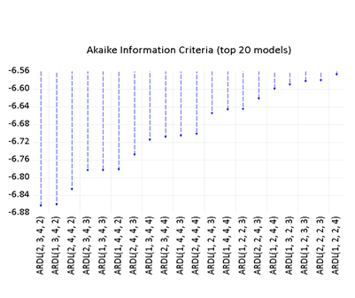
Model Selection method: AIC
Maximum dependant lags: 2 (Automatic selection)
DYnamic Regressors (4 lags Automatic): LI (income), LE (energy use), LFDI (FDIinflow)
Selected Model: ARDL (2,3,4,2)
R squared: 0.999375
Adjusted R squared: 0.998501
S.E of regression: 0.006788
Sum squared resid: 0.000461
Log likelihood: 100.7943
F-stat: 1142.911
Prob (F-stat): 0.00000
| Variable | Coefficient | Std. Error | t-stat | Prob |
| LC(-1) | 0.5364 | 0.1653 | 3.2441 | 0.0088 |
| LC(-2) | 0.1340 | 0.1436 | .09332 | 0.3727 |
| LI | -0.1114 | 0.1733 | -0.6430 | 0.5347 |
| LE | 1.026 | 0.1985 | 5.1677 | 0.0004 |
| LFDI | -0.015 | 0.0007 | -2.0322 | 0.0495 |
* LI (income), LE (energy use), LFDI (FDIinflow)
99% of r-squared value and adjusted r-squared value tells us this is a best fitted model. Prob(F stat) of 0.00 which is below 5% indicates this is a highly significant model.
The p value for LI (income) is 0.534 which is above 5% significance level, which makes the result insignificant. The t statistic of -0.6403 is also not above 2 in absolute form, indicating the value is insignificant.
In case of LE (energy consumption), the t stat of 5.16 and p value below 5% level of 0.0004 shows the result is highly significant. The coefficient of LE tells us that a 1% rise in energy consumption leads to co2 emissions to also rise by 1.026% in the short run assuming other variables are constant or unchanged.
P value and T-stat of LF (FDI inflow) provide evidence for significance at 5% level. In the short run, a 1 percent growth in FDI inflow value leads to a 0.015% fall in co2 emissions, ceteris paribus. This is possible when the inflow of investment is used for businesses that avoid environmental pollution, or are environmentally sound and follow the environmental guidelines and laws. When FDI is reducing co2 emissions, it may imply that these new foreign investments are greener and are replacing the businesses that previously emitted higher levels of co2 emissions.
The short run results show us that 2 out of the 3 explanatory variables are significantly affecting the dependent variable or co2 emissions.
In other words, rising income does not cause a significant change in the air quality in the country in the short run.
We have selected the Akaike info criterion for lag selection here. The lag selection criteria is shown below.
BOUNDS TEST
The ARDL bounds test approach has been used here to test for the long run links between variables. It’s a cointegration technique which was designed by Pesaran et al. (2001). This test is a useful tool regardless of whether series are integrated of order I(0) or I(1). Empirical results also show that this approach is better and gives consistent outcomes in case of a small sample.
LC (co2 emission) : dependant variable
Method: ARDL Long run form and bounds test
Sample: 1986-2014
Selected Model: ARDL (2,3,4,2)
25 observations after adjustments
LEVELS EQUATION
Case 3: Unrestricted Constant and No Trend
| Variable | Coefficient | Std. Error | t-stat | Prob |
| LI | -0.1187 | 0.3974 | -2.0086 | 0.0313 |
| LE | 1.1318 | 1.1490 | 0.9850 | 0.3478 |
| LF | 0.07167 | 0.02390 | 2.9976 | 0.0134 |
| C | -3.3493 | 1.37329 | -2.4388 | 0.0349 |
*LI (income) , LE (energy used), LFDI (FDI inflow)
EC=LC-(-0.118*LI+1.131*LE+0.071*LF-3.3493)
| F bounds test | Null hypothesis: No levels relationship | |||
| Test Statistic | Value | Significance | I(0) | I(1) |
| F statistic | 8.4517013 | 10% | 2.37 | 3.2 |
| 5% | 2.79 | 3.67 | ||
| 2.5% | 3.15 | 4.08 | ||
| 1% | 3.65 | 4.66 | ||
The F bounds value of 8.4517013 is higher than the upper value, I(1) of 4.66 at 1% significance level. Thereby we can say there is a long run relationship. The table above this shows the coefficients of long run relationships.
The results of LE are insignificant since the P values are higher than 0.05. T stats are also below 2 in absolute form.
In the case of LFDI and LI, the results can be interpreted since it is significant.
A 1% rise in inflow of FDI in Bangladesh causes a 0.07167% increase in the co2 emissions in the long run, ceteris paribus.
For income per capita, a 1% rise in income will lead to a 0.1187% fall in co2 emissions in the long run. A negative correlation exists.
| Breusch-Goldfrey Serial Correlation LM Test
Null Hypothesis: No serial correlation upto 2 lags |
|||
| F stat | 1.356 | Prob F (2,8) | 0.3110 |
| Obs R squared | 6.330 | Prob. Chi-Square(2) | 0.0422 |
The chi square value being less than 0.05 stipulates that we can reject the null hypothesis of no serial correlation. Meaning that serial correlation exists in our model.
In time series data, serial correlation occurs when a variable and it’s own lagged version are related with each other over time periods. Recurring patterns often exhibit serial correlation at times when the measure of a variable affects its future value.
The concept originated through use in the engineering field to understand the way computer signals or a radio wave may vary over time when compared to itself. Popularity of the concept grew later in the economics field when economists, experts and econometrics students used the concept to study data in time series.
which indicates that our model is a stable one.
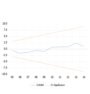
Cusum test is used to examine the uniformity of the coefficients (β) in a multiple linear regression model. It is used to analyse models which are in the form y = Xβ + ε. A series of sums, or sums of squares, of recursive residuals computed repeatedly from the nested subsamples of data are used to make inferences. The null hypothesis says that the coefficients are constant.
If values of the sequence are found to be outliers, it indicates a possibility of structural change in the model over time.
Now we have the cusum tests here above, which tells us whether our model is a stable one or not. The blue line, cusum line is between the 5% significance curves, which indicates that our model is a stable one.
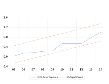
Above we can see the CUSUM of Squares graph, which also exhibits a stable model structure.
However, our model also has serial correlation which needs to be fixed.
For that, we estimate this through OLS and add an error correction term.
| Dependant variable: D(LC)
Method: Least squares Sample : 1991 2014 24 observations after adjustments |
||||
| Variable | Coefficient | Std Error | T-stat | Prob. |
| C | 0.037 | 0.028 | 1.309 | 0.2170 |
| D(LC(-1)) | -0.387 | 0.839 | -0.461 | 0.6537 |
| D(LC(-2)) | 0.314 | 0.358 | 0.876 | 0.3995 |
| D(LI(-1)) | 0.761 | 0.295 | 2.580 | 0.0255 |
| D(LI(-2)) | -0.140 | 0.501 | -0.279 | 0.7850 |
| D(LI(-3)) | -0.085 | 0.316 | -0.270 | 0.7919 |
| D(LE(-1)) | -0.169 | 0.667 | -0.254 | 0.8039 |
| D(LE(-2)) | -0.727 | 0.711 | -1.022 | 0.3286 |
| D(LE(-3)) | -0.163 | 0.520 | -0.313 | 0.7597 |
| D(LE(-4)) | -1.300 | 0.430 | -3.023 | 0.0116 |
| D(LF(-1)) | -0.016 | 0.032 | -0.527 | 0.6081 |
| D(LF(-2)) | 0.031 | 0.016 | 1.930 | 0.0789 |
| ECT(-1) | -1.219 | 1.003 | -1.215 | 0.2496 |
After this we add the error correction term (ecm or the residual). It is used to compute the pace of adjustment towards overall equilibrium.
However the results depict that the ECT is not significant here, as p value is above 0.05.

A stability test was run after generating the ECT. The cusum test here shows the model is not stable.
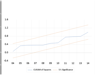
However, the cusum squared test results depict that it is a stable model.
After adding the ECT, we run the LM test again to test for serial correlation.
| Breusch-Goldfrey Serial Correlation LM Test: Null Hypothesis: No serial correlation at upto 2 lags | |||
| F-stat | 0.437854 | Prob. F(2,9) | 0.6585 |
| Obs* R-squared | 2.128149 | Prob. Chi-Square(2) | 0.3450 |
Now the new chi square value is 0.345. We cannot reject the null hypothesis.
Thus we accept a null hypothesis of no serial correlation upto 2 lags.
Now our model is free from serial correlation.
CONCLUSION AND POLICY IMPLICATIONS
Our analysis outcomes using ARDL method exhibit a negative or inverse connection among influx of FDI and air pollution in the short run. Whereas in the big picture or the long run, a positive relationship is found.
This tells us that the inflow of investment lowers the quantity of co2 emitted slightly in the short run. This may happen when foreign investors focus on environmental sustainability and aim to perform business operations according to environmental regulations. However, overall pollution levels rise again with rising investment in the long run.
Policymakers should take this effect into account to regulate foreign investors and their business management systems to strictly follow some developed guidelines.
Our analysis did not show any significant effect that income may have on the co2 emission level in the short term. In the long run, there is a negative relationship between the variables.
Moreover, air pollution increases more than proportionately with energy consumption in the short run. However, no significant effect in the long run could be detected in our analysis.
We can infer here that other renewable sources of energy should be adapted immediately. Sustainability should be maintained firmly while energy consumption rises, since rising use of energy is inevitable with growth and development. If the environment continues to be subjected to constant and routine degradation, human beings will have to endure all consequences including adverse effects on health, agriculture, natural disasters, irregular climate, weather shocks and so on. These impacts in turn affect the economic activities of a country. Hence, taking sustainability into account is of supreme importance in this time and age before it gets too late.
It can be concluded that since no significant relationship between income and co2 emission could be identified in the short run, no EKC relationship can be found for Bangladesh between the time period of 1986 to 2014. However, even if EKC exists for Bangladesh it may be over a greater period of time, and the time period 1986-2014 may be inferred to be the time period where the country experiences the turning point or initial downward sloping portion of EKC as suggested by long run results.
In any case, this thesis paper has not been able to prove the existence of the entire Environmental Kuznets Curve (upward sloping which later becomes downward sloping) through data analysis.
Hypothesis:
H0 (null hypothesis): there is no (EKC for Bangladesh) relationship between income increase and co2 emissions
H1(alternate hypothesis) : H0 is not true
Here, we accept the null hypothesis.
REFERENCES
- Miah, M., Masum, M., Koike, M., Akther, S., & Muhammed, N. (2011). Environmental Kuznets Curve: the case of Bangladesh for waste emission and suspended particulate matter. The Environmentalist, 31(1), 59-66. https://doi.org/10.1007/s10669-010-9303-8
- Jahangir Alam, M., Ara Begum, I., Buysse, J., & Van Huylenbroeck, G. (2012). Energy consumption, carbon emissions and economic growth nexus in Bangladesh: Cointegration and dynamic causality analysis. Energy Policy, 45, 217-225. https://doi.org/10.1016/j.enpol.2012.02.022
- Jungho, B., & Won W., K. (2009). A Dynamic Approach to the FDI-Environment Nexus: The Case of China and India. East Asian Economic Review, 13(2), 87-106. https://doi.org/10.11644/kiep.jeai.2009.13.2.202
- Shafik, N. (1994). Economic Development and Environmental Quality: An Econometric Analysis. Oxford Economic Papers, 46, new series, 757-773. Retrieved December 23, 2020, from http://www.jstor.org/stable/2663498
- Angelsen, A., & Kaimowitz, D. (1999). Rethinking the Causes of Deforestation: Lessons from Economic Models. The World Bank Research Observer, 14(1), 73-98. https://doi.org/10.1093/wbro/14.1.73
- Neumayer, E. (2000). Trade and the Environment: A Critical Assessment and Some Suggestions for Reconciliation. The Journal Of Environment & Development, 9(2), 138-159. https://doi.org/10.1177/107049650000900203
- Amin, S., Morshed, M., &Porna, A. (2016). Energy Consumption, Economic Growth & Environmental Quality: A Causal Relationship Revisited for the Bangladesh Economy. International Review Of Business Research Papers, 12(2), 183-203. https://doi.org/10.21102/irbrp.2016.09.122.12
- Alam, J. (2014). On the Relationship between Economic Growth and CO2 Emissions: The Bangladesh Experience. IOSR Journal Of Economics And Finance, 5(6), 36-41. https://doi.org/10.9790/5933-05613641
- Baek, J., & Choi, Y. (2017). Does Foreign Direct Investment Harm the Environment in Developing Countries? Dynamic Panel Analysis of Latin American Countries. Economies, 5(4), 39. https://doi.org/10.3390/economies5040039
- Jahangir Alam, M., Ara Begum, I., Buysse, J., & Van Huylenbroeck, G. (2012). Energy consumption, carbon emissions and economic growth nexus in Bangladesh: Cointegration and dynamic causality analysis. Energy Policy, 45, 217-225. https://doi.org/10.1016/j.enpol.2012.02.022
- Holtz-Eakin, D., & Selden, T. (1995). Stoking the fires? CO2 emissions and economic growth. Journal Of Public Economics, 57(1), 85-101. https://doi.org/10.1016/0047-2727(94)01449-x
- Friedl, B., & Getzner, M. (2003). Determinants of CO2 emissions in a small open economy. Ecological Economics, 45(1), 133-148. https://doi.org/10.1016/s0921-8009(03)00008-9
- Arrow, K., Bolin, B., Costanza, R., Dasgupta, P., Folke, C., & Holling, C. et al. (1996). Economic growth, carrying capacity, and the environment. Environment And Development Economics, 1(1), 104-110. https://doi.org/10.1017/s1355770x00000413
- Chandra Ghosh, B. (2014). Economic Growth, CO2 Emissions and Energy Consumption: The Case of Bangladesh. International Journal Of Business And Economics Research, 3(6), 220. https://doi.org/10.11648/j.ijber.20140306.13
- Jungho, B., & Won W., K. (2009). A Dynamic Approach to the FDI-Environment Nexus: The Case of China and India. East Asian Economic Review, 13(2), 87-106. https://doi.org/10.11644/kiep.jeai.2009.13.2.202
- Kim, Hyun & Baek, Jungho. (2011). The Environmental Consequences of Economic Growth Revisited. Economics Bulletin. 31. 1198-1211.
- Sustainable development cooperation framework – the United Nations in … (n.d.). Retrieved from https://bangladesh.un.org/en/download/89263/159595
- BUDGET REPORT 2021-22 Finance Division, Ministry of Finance Government of the People’s Republic of Bangladesh CLIMATE FINANCING for SUSTAINABLE DEVELOPMENT.
- Bangladesh Bureau of Statistics. (2021). Statistical Yearbook of Bangladesh. Dhaka: Bangladesh Bureau of Statistics.
- Government of Bangladesh. (2010). Renewable Energy Policy of Bangladesh. Dhaka: Ministry of Power, Energy, and Mineral Resources.
- Government of Bangladesh. (1992). National Environment Policy. Dhaka: Ministry of Environment and Forests.
- Hossain, M. (2015). Environmental Protection Policies and Their Implementation in Bangladesh: An Overview. Journal of Environmental Science and Natural Resources, 8(1), 69-75.
- Islam, M. M., & Rahman, M. M. (2017). Waste Management in Bangladesh: Current Status and Future Challenges. Waste Management & Research, 35(6), 581-590.
- Bangladesh Ministry of Environment, Forest and Climate Change. (2018). National Environment Policy. Retrieved from http://www.moef.gov.bd/sites/ default/files/files /moef.portal.gov.bd /policies/ce43 b8ed_9f05_4f26_8246_5835b5a0b0a2/National%20 Environment%20Policy.pdf
- Bangladesh Environmental Lawyers Association. (2017). Environmental Laws and Regulations in Bangladesh. Retrieved from http://www.bela-bd.org/environmental-laws-and-regulations-in-bangladesh/
- Food and Agriculture Organization of the United Nations. (2016). State of the World’s Forests 2016. Retrieved from http://www.fao.org/3/a-i4793e.pdf
- International Renewable Energy Agency. (2019). Renewable Energy Country Profile: Bangladesh. Retrieved from https://www.irena.org/-/media/Files/IRENA/Agency/Publication/ 2019/Apr/IRENA_RE_Country_Profile_Bangladesh_2019.pdf
- The World Bank. (2018). Bangladesh – Improving Municipal Solid Waste Management Project. Retrieved from https://projects.worldbank.org/en/projects-operations/project-detail/P158421