Exploring the Dynamic Landscape of Economic Dispatch: A Comprehensive Review of Stochastic Programming Techniques

Exploring the Dynamic Landscape of Economic Dispatch: A Comprehensive Review of Stochastic Programming Techniques

D. Punsara Colambage¹, W.D. Anura S. Wijayapala², Tilak Siyambalapitiya³

^1,2Department of Electrical Engineering, University of Moratuwa, Sri Lanka

³Ceylon Electricity Board, Colombo 02, Sri Lanka.

DOI: https://dx.doi.org/10.47772/IJRISS.2025.90400141

Received: 30 March 2025; Accepted: 03 April 2025; Published: 02 May 2025

ABSTRACT

Ensuring the provision of high-quality and continuous power at an affordable rate stands as the primary objective of power systems. To achieve this goal, utilities devise economic dispatch schedules for each quarter-hour time slot, leveraging stochastic programming methodologies. This becomes imperative due to the inherent uncertainty associated with renewable energy sources, heavily reliant on weather and climate conditions. Dynamic Programming, Stochastic Dynamic Programming, and Stochastic Dual Dynamic Programming techniques are deployed to formulate real-time economic dispatch schedules. Notably, while cost remains a pivotal factor, the emphasis shifts towards economic value, particularly water value, during the dispatch process. Various methodologies have been introduced to ascertain the optimal economic dispatch schedule, considering the dynamic landscape of economic dispatch. This landscape plays a crucial role in the design, analysis, planning, and modelling of smart energy systems, facilitating informed decisions for the green transformation of energy supply and demand systems towards future smart renewable energy solutions. This research paper offers a comprehensive literature review of stochastic programming techniques applied in economic dispatch, shedding light on their implications for smart energy systems.

Keywords: Economic Dispatch, Stochastic, Water Value, Dynamic Programming

INTRODUCTION

In the intricate dance of managing a power system, utility operators face the daunting task of orchestrating the ideal blend of power plants to meet fluctuating electricity demands. At the heart of their challenge lies the short-term optimisation puzzle: how to meticulously schedule generation to minimise total costs while adhering to a myriad of constraints. With an eye toward efficiency and sustainability, power system owners constantly seek to optimise the balance between constructing new, state-of-the-art power plants and retiring older, less efficient ones.

Responsibility for meeting electricity demand rests squarely on the shoulders of the utility company, underscoring the critical importance of ensuring that global generation matches forecasted demands on a quarter-hourly basis. Unit Commitment and Economic Dispatch emerge as pivotal factors influencing generation costs. Unit Commitment involves the strategic decision-making process of determining when and which generating units at each power station to activate or deactivate, while Economic Dispatch entails fine-tuning individual power outputs to align with scheduled generating unit capacities at each time interval [1][2].

At its core, the unit commitment process is driven by the overarching objective of minimising operating costs while satisfying all operational and systemic constraints. This intricate ballet of generation scheduling involves meticulous planning of startup, shutdown, and power levels for each unit over a defined scheduling horizon. The aim is to strike a delicate balance, minimising operational expenses, startup, and shutdown costs while ensuring seamless continuity of power supply [3].

Delving deeply into the concept, Unit Commitment intricately navigates the optimal scheduling and production levels of each generator unit within a power system for a given time frame, meticulously balancing operational constraints and equipment requirements. On one front, it meticulously delineates the commitment status of generators—whether they are poised to be activated or remain dormant—during the corresponding period. Subsequently, Economic Dispatch steps in to meticulously ascertain production levels within smaller time intervals [4][5].

Traditionally, Unit Commitment primarily addresses security-based constraints such as line outages and transmission line capacities, often overlooking network constraints. Conversely, from the perspective of market operators, Unit Commitment seamlessly integrates to minimise costs and maximise the benefits of generation targets [6].

Economic Dispatch unfolds into deterministic and stochastic realms, navigating uncertainties stemming from forecast deviations and equipment reliability issues. Fluctuations in forecasts can trigger load variations, compounded by the intermittent and volatile nature of renewable energy generation, leading to forecast errors with increasing renewable energy penetration. To minimise generation costs while meeting consumer electricity demands, it becomes imperative to strategically determine the output capacities and commitment statuses of each power plant, accounting for forecasts and constraints. Subsequently, a secondary dispatch round becomes indispensable to reconcile disparities between actual and forecasted demand [7][8].

In essence, addressing power system optimisation poses a significant challenge due to its capacity to encompass diverse technical, economic intricacies, and uncertainties. Attempting to incorporate all these elements into a single problem becomes computationally infeasible. Consequently, a typical approach involves considering a hierarchy of problems that tackle various time scales and perspectives. These include short-term dispatch (spanning a few days or weeks), mid-term operational planning (covering 1-2 years), and long-term operational planning (spanning 3-5 years). The outcomes derived from a long-term model can then be integrated into a model with a shorter horizon, but with more detailed considerations in other aspects of modelling [9].

Dynamic programming (DP) proves to be a potent method for addressing optimisation issues characterised by overlapping subproblems and optimal substructure. The enhanced forms of Dynamic Programming, namely Differential (or incremental) Dynamic Programming (DDP) and Discrete Differential Dynamic Programming (DDDP), contribute to achieving more precise outcomes in problems with overlapping subproblems and optimal substructure [10][11]. Various literature sources propose distinct methodologies; however, this discussion focuses on several successful and applicable approaches. One of these mathematical techniques were employed by a Sri Lankan Engineer, P.J. Perera, in the 1980s to establish a methodology for water resources planning [12].

J. Perera’s model of Dynamic Programming Techniques for Water Resource Planning

Dynamic Programming (DP) techniques which are based on Bellman’s Principle of Optimality might be conveniently used in water resources optimisation due to stage-by-stage applicability. The basic idea of Bellman’s Principle states that in a decision policy, whatever the initial states and the initial decisions are, the remaining decisions must constitute an optimal policy regarding the states resulting from the initial decision [12].

Basic derivation for the deterministic case

Dynamic Programming for Reservoir Control

Where,

• \( F \) – Objective function
• \( f(x_t, u_t) \) – Function representing the combined effect of the system transformations succeeding from an initial state vector \( x_0 \) to a final state vector \( x_T \) resulting from a series of decision vectors \( u_t \)
• \( g_t(x_t, u_t) \) – The return at stage \( t \) with respect to the state vector \( x_t \) and the decision vector \( u_t \)
• \( U_t \) – The administrative domains for decision vector \( u_t \)
• \( x_t \) – State vector for stage \( t \)

A cost minimisation, additive properties prevail in the function can be expressed as,

\[
J_t(x_t) = \min_{u_t \in U_t} \left[ g_t(x_t, u_t) + J_{t+1}(x_{t+1}) \right]
\]

Where,

• \( S_t \) – Reservoir storage at stage \( t \)
• \( R_t \) – Release of this storage at stage \( t \)
• \( J_t(x_t) \) – Minimum cost for operating the system from an initial state \( x_t \) to some final state

By the definition,

\[
J_t(x_t) = \min_{u_t \in U_t} \left[ g_t(x_t, u_t) + J_{t+1}(x_{t+1}) \right] \tag{1}
\]

Equation (1) represents the Dynamic Programming recursive algorithm, from an initial state vector  to a final state . Depending on whether the initial state or the final state is known, the algorithm could be applied in a forward or backward manner. If both states are known, it could be applied either way. Fig. 01 gives a graphical representation of the DP operation, when applied to a reservoir control problem.

Fig 01. Dynamic Programming Operation to Control the Reservoir Problem

Basic Derivation for Stochastic Case

The stochastic element in reservoir operation is streamflow, and once this effect is introduced, the return function becomes dependent upon both storage \( S_t \) and inflow \( Q_t \), in addition to the decision variable \( R_t \).

Equation (1) can be revised as,

\[
J_t(S_t) = \min_{R_t} \sum_{Q_t} p(Q_t) \left[ g_t(S_t, Q_t, R_t) + J_{t+1}(S_{t+1}) \right]
\]

Where,

• \( p(Q_t) \) – The probability density function of \( Q_t \) for a discrete probability distribution

Where,

• \( Q_t^i \) – Discretisation of the streamflow at stage \( t \)
• \( p_i \) – Probability of occurrence
• \( N \) – Total number of discretisation

Markov Chains and Serial Correlation

A Markov Chain of the first order is defined as a sequence of events \( \{X_t\} \) of discrete random variables, with the property that the conditional distribution of \( X_t \), given \( X_{t-1}, X_{t-2}, \dots \), depends only on the value of \( X_{t-1} \), but not further. For any state values of \( X_t \) belonging to the discrete state space,

\[
P(X_t = x_t | X_{t-1} = x_{t-1}, X_{t-2} = x_{t-2}, \ldots) = P(X_t = x_t | X_{t-1} = x_{t-1})
\]

When a streamflow of a certain month is independently analysed using recorded previous data, a certain probability distribution could be derived for its representation. However, this distribution is usually conditional upon the actual streamflow of the previous month, as in the case of the occurrence in a first-order Markov Chain. The basic derivation for the stochastic case with the introduction of this serial correlation is as follows:

\[
J_t(S_t, Q_{t-1}) = \min_{R_t} \sum_{Q_t} p(Q_t | Q_{t-1}) \left[ g_t(S_t, Q_t, R_t) + J_{t+1}(S_{t+1}, Q_t) \right]
\]

Where,

• \( p(Q_t^i | Q_{t-1}) \) – The conditional probability of streamflow at stage \( t \) falling into the discretisation \( Q_t^i \), given inflow \( Q_{t-1} \) at stage \( t-1 \)

It is evident that no unique optimal trajectory exists when serial correlation is considered.

Different Dynamic Programming Techniques

Where,

m_q – number of occurrences of the streamflow in month n-1 within the class interval q

m_p – within the set of occurrences of m_q, the subset of occurrences of streamflow in month

n within the interval p

For k inflow intervals, the expectation of the inflow I_n for a certain month n, given the actual inflow interval of the previous month as q is,

for equal probability intervals.

A transition probability matrix can be defined for the streamflow of any two adjoining months n and n+1 such that,

The Mid-Term schedule with deterministic inflows       

This is implemented either on a monthly or weekly basis. The inflow regimes at various dam sites are found for various hydro-conditions using probability analysis and are classified under various dry-conditions. For example, 60%- dry would mean that the inflow will be greater or equal to the corresponding value for 60% of the time. It is illustrated by  in the inflow- duration curve given in Fig. 02.

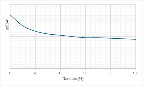
Fig 02. Flow Duration Curve

The input of inflows to the model can be given as a combination of these dry conditions for 12 months. The model uses DDDPSA to arrive at the optimal trajectories for the reservoirs.

Evaluation of the return function

To obtain the thermal plant costs for each trajectory of the state variables, the load duration curve for that month is probabilistically simulated with the corresponding hydro energy included. The hydro components groups into the two basins of Mahaweli and Kelani rivers are fitted using Jacoby’s method with zero outages are assumed. For thermal plants, forced and scheduled outages are considered, and the plants are probabilistically stacked on the load duration curve in the order of their increasing operating cost.

Irrigation requirements          

Irrigation only exists in the Mahaweli basin, at Polgolla and Minipe. The irrigation requirements off Polgolla are specified at three sites of Bowatenna, Elahera and Angammedilla. These requirements are given monthly at these sites. If an irrigation deficit is to be affected at Polgolla in an annual basis, there are numerous combinations possible in the adjusted diversions at these sites, and it should be initially investigated as to which distribution of the actual diversions are more realistic in actual practice. The DP routine can be made sensitive to irrigation diversions by the introduction of a penalty cost in the case of an irrigation deficit.  The form of this penalty should incorporate not only the limitation of the total diversion deficits, but also how these deficits are distributed within the year.

For example, a total annual deficit of 100 MCM at Polgolla can give rise to a deficit at Bowatenna of 50 MCM in January and 50 MCM in December (leaving aside Elehera and Amgammedilla) or a 25 MCM deficit in January and a 75 MCM deficit in December. Since the diversion requirements at Bowatenna are 75 MCM for all months, the former case seems more appropriate in a practical sense as the optimising model does not consider the diversion storages as state variables. The introduction of a linear irrigation penalty can give rise to inappropriate monthly irrigation diversions because the results can exhibit insensitivity to the diversion pattern within the year. What is essentially required is the capability of the model to meet the requirements within the constraints imposed by the inflows, such that if there should be any deficits, these to be allocated monthly rather than in an annual basis. This is accomplished by introducing an exponential irrigational penalty rather than a linear penalty. For the example considered earlier, a linear penalty will give rise to identical irrigation penalty costs for the two cases, whereas the introduction of an exponential penalty of the form,

cost=EXP(deficit each month)

will minimise the penalty for the former case. The following expression illustrates this,

EXP(50)+EXP (50)=EXP(25)+EXP(75)

even though,

50 + 50 = 25 + 75

This penalty cost of course will have no physical meaning, but when added to the thermal costs for the various reservoir trajectories in the DP exercise, the resulting optimal trajectories will satisfy the irrigation in the most appropriate way monthly. This exponential irrigation penalty factor can also be used to enforce the trade-off between irrigation and power. A very low penalty will enforce negligible influence on irrigation deficits and in effect will optimise for the power only, whereas with a high penalty, the vice-versa will occur. Since quantification of actual irrigation losses are quite complex and inaccurate, under normal running the model is made to assume a very high penalty factor for irrigation deficits whereby the thermal cost is minimised only after meeting the irrigation requirements within the constraints of the inflows.

The mid-term schedule with stochastic inflows

A composite basin representation is used in the study due to the excessive number of state variables existent in the system. The composite representation agglomerates the reservoirs in each basin into one equivalent energy storage entity and an associated generating plant. The composite model is based on a single measure of potential energy which is indicative of the system’s generating capability. The one-dam representation of the multi-reservoir system in effect receives, stores and releases potential energy when operative in the DP routine. The inflows also should be represented by the potential energy input into the system. The dependence between the potential energy outflow and the electrical energy generated is given by the generation function of each composite basin [4].

The composite model is most applicable when the sequence of monthly decisions on the total hydro generation is of greater economic significance than the allocation of these among the various hydro plants. The decomposition of this total generation to those of the individual plants depends on the initial derivation of the generation function. Therefore, it is of basic importance to maintain as far as possible a consistent approach to this problem with that applied for achieving the main objective of the study.

Generation Functions

The power generation of a hydro plant as a function of the released water depends on the plant head and the overall plant efficiency. This is given by,

Q_max is determined by the maximum turbine capacity, and H_max occurs when the reservoir level is at its maximum. If Q> Q_max, there will be no further contribution to the generation.

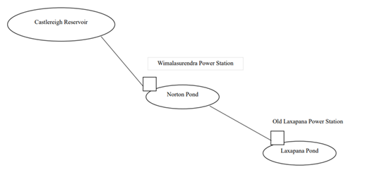
Fig 03. Cascadic structure of Laxapana Hydro Complex in Sri Lanka

Notations

• \( t \): Time interval (hour) index
• \( T \): Total number of time intervals (scheduling horizon)
• \( D_t \): Total demand (MW)
• \( P^{\text{thermal}}_t \): Total thermal power supply
• \( P^{\text{hydro}}_t \): Total hydro power supply
• \( N \): Number of available thermal plants
• \( U_i \): Number of units in \( i^{th} \) thermal plant
• \( U_j \): Number of units in \( j^{th} \) thermal plant
• \( C_i \): Commitment state of \( i^{th} \) thermal plant
• \( S_{i,n,t} \): Status of \( i^{th} \) plant, \( n^{th} \) unit at \( t^{th} \) state
• \( x_{i,n,t} \): Discrete status of \( i^{th} \) plant, \( n^{th} \) unit
• \( M_{i,n} \): Maintenance state of \( i^{th} \) plant, \( n^{th} \) unit
• \( P_{i,n} \): Power output of \( i^{th} \) plant, \( n^{th} \) unit (MW)
• \( H_{j,t} \): Power output for the reservoir \( j \) during hour \( t \)
• \( C_i(P) \): Cost function of \( i^{th} \) plant in LKR/hr
• \( P^{\max}_{i,n} \): Max power output of \( i^{th} \) plant, \( n^{th} \) unit
• \( P^{\min}_{i,n} \): Min power output of \( i^{th} \) plant, \( n^{th} \) unit
• \( P^{\max}_{j} \), \( P^{\min}_{j} \): Max/Min output of hydro unit \( j \)
• \( R_{i,n} \): Ramp rate (MW/hr)
• \( UT_{i,n} \): Minimum up time (hrs)
• \( DT_{i,n} \): Minimum down time (hrs)
• \( RH_{i,n} \): Reserved hours (hrs)
• \( SC_{i,n} \): Start-up cost (LKR)
• \( SHC_{i,n} \): Shutdown cost (LKR)
• \( TC_{i,t} \): Total thermal cost at \( t^{th} \) hour
• \( D^{\text{total}}_t \): Total demand when units dispatched at \( t \)
• \( D^{\text{remain}}_t \): Remaining demand to dispatch at \( t \)
• \( DT_{i,n,t} \): Consecutive downtime of unit \( n \) of plant \( i \) at \( t \)
• \( CL^{\max} \): Maximum capacity limit percentage

Objective Function

The goal is to minimize the total cost of generation while meeting demand and adhering to constraints:

\[
\min \sum_{t=1}^{T} \sum_{i=1}^{N} C_i(P_{i,t}) + \text{Startup/Shutdown Costs}
\]

System Constraints

Demand Satisfaction

\[
\sum_{i=1}^{N} \sum_{n=1}^{U_i} P_{i,n,t} + \sum_j H_{j,t} = D_t, \quad \forall t
\]

Technical Limits

\[
P^{\min}_{i,n} \leq P_{i,n,t} \leq P^{\max}_{i,n}
\]

Startup/Shutdown Costs

Included in objective as \( SC_{i,n} \) and \( SHC_{i,n} \)

Spinning Reserve

Must satisfy system reserve margin.

Minimum Uptime/Downtime

– Varies by plant type (coal, combined cycle, nuclear).
– Hydro: negligible due to fast start/stop.

Ramp Rate

\[
|P_{i,n,t} – P_{i,n,t-1}| \leq R_{i,n}
\]

Thermal Plant Cost Function

No quadratic term in Sri Lankan context. Costs are assumed linear:
\[
C_i(P) = a_i P + b_i
\]

Algorithm (Metro Dispatch)

Input:

• Half-hourly demand curve
• Available plant and cost details
• Maintenance schedule
• Initial ON/OFF status, hours stopped, running units

Step 1: Generate Initial Schedule

Sort plants by ascending unit cost. Combined cycle plants use average cost.

Step 2: Generate Options

\[
\text{Options} = 2^N
\]

Remove options violating:
\[
\text{Total Min Load} < D_t < \text{Total Max Load}
\]

Step 3: Commit Plants

Plants, not units, are selected. All committed plants dispatch at least minimum load.

Transitions

• Transition 1: OFF → ON
• Transition 2: ON → OFF
• Transition 3: ON → ON
• Transition 4: OFF → OFF

Total cost for option = energy cost + transition cost

Short-Term Forecasting

• Time series, regression, AI, hybrid models

Accuracy measured using:
\[
\text{MAPE} = \frac{1}{n} \sum_{t=1}^{n} \left| \frac{A_t – F_t}{A_t} \right| \times 100
\]

Water Value Models

Fuel cost is key for thermal plant operation:
\[
\text{Minimize } C = \sum_{t} \sum_j c_j P_{j,t}
\]
Subject to:
\[
0 \leq P_{j,t} \leq P^{\max}_j
\]
\[
\sum_j P_{j,t} = D_t
\]

Determining the power plant combination to achieve the required load with minimising the fuel cost

Immediate Cost Function (ICF) and Future Cost Function (FCF)

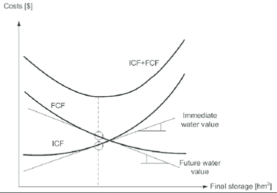
Hydropower plants utilise their stored water resources to avoid the fuel expenses of thermal power plant units. The availability of hydropower plants depends on the water storage of reservoirs. The main decision to be made at the scheduling stage is to release the required amount of water by evaluating immediate financial gain and the expected value of water in the future. The expected value of the water in the future is represented by a function of inflow, reservoir level, and time. The ICF (Inflow, Cost, Function) has a relationship with the cost of thermal energy at the t stage. When the final storage is gradually increasing, only a small amount of water is available for electricity generation at the same stage. As a result, more thermal energy is required, leading to an increase in cost. By the way, the FCF (Future Cash Flow) associated with predicted thermal expenses from (t+1) to the ending point of the period will decrease due to the availability of more water for future energy production, as shown in Fig. 04 [16] [17].

Optimisation Algorithm

Where,

• \(\bar{p}_s\) – average short price in the week
• \(\tilde{p}_s\) – normalised value of \(p_s\)
• \(\alpha\) – auto correction coefficient determined from the future function
• \(\epsilon\) – normal random variable

Principle of Mass Production Theory

When the utilised capacity is increasing, fixed cost is declined and variable cost increases.

• \(C_{\text{avg}}\) – total average cost
• \(C_f\) – total fixed cost
• \(Q\) – production quantity
• \(C_v\) – total variable cost

To obtain the variable cost of a thermal power plant, a specific heat rate curve is used. The specific heat curve provides information on the necessary heat energy required for generating one unit of electrical energy.

• \(P_t\) – Thermal power plant production
• \(a\) – coefficient
• \(f(P_t)\) – input–output curve
• \(F(P_t)\) – fuel cost function
• \(b\) – fuel cost coefficient

Water Value Deterministic Function

• \(C_w\) – function cost curve for water value
• \(P_d\) – power needed in system
• \(V_r\) – reservoir level
• \(V_p\) – planned reservoir level

System Production Optimisation

Where,

• \(C_t\) – immediate cost of thermal power plants operating cost in stage \(t\)
• \(C_f^h\) – future cost of hydro power plant
• \(\beta_k\) – production coefficient of reservoir \(k\)
• \(W_k\) – water value function of the reservoir
• \(V_k^t\) – reservoir volume at the end of stage \(t\)
• \(E\) – power exchange

For the easiness of understanding, the function can be modified as:

• \(C_t^T\) – cost of thermal power plant
• \(C_t^H\) – cost of hydro power plant
• \(E_t\) – energy sold or bought on power exchange

Summation of power production and energy exchange has to be equal to the planned load for each period.

To achieve the maximum financial benefits, …

CONCLUSION AND DISCUSSION

Cost accounting serves as a multifaceted method encompassing the accumulation, classification, summarisation, and interpretation of information crucial for operational planning, control, and strategic decision-making [18]. A primary aim of cost accounting lies in determining optimal selling prices. Beyond this, its objectives extend to enhancing control efficiency, facilitating financial statement preparations, and laying the groundwork for operational policies, such as delineating cost-volume-profit relationships and evaluating the feasibility of outsourcing from external suppliers. In the realm of electricity generation, these objectives align with tasks like tariff formulation, strategic decisions regarding the establishment of pump storage power plants, importing power from neighbouring countries via tie-lines, and electrification initiatives [19]. Broadly defined, cost signifies the expenditure associated with production, calculated either through actual or notional values. For power plants, unit cost considerations encompass operational and maintenance expenses, fuel costs, and depreciation. However, the valuation of energy units extends beyond these factors to include opportunity costs, reflecting the value in terms of the unit cost of the next best alternative [19] [20][21].

The primary objective of optimising the operational schedule of a hydrothermal system is to define efficient operational strategies for each planning stage and corresponding system states to achieve targeted power generation from each power plant. These strategies aim to minimise operational costs over time, including fuel expenses and penalties for load supply failures, while considering constraints such as stored water resources. The dynamic nature of water resource availability, influenced by present and future variations in value, underscores the importance of effectively managing reservoir levels [22][23]. This management involves linking operational decisions at each stage with their future implications, particularly regarding the depletion of hydroelectric energy and the potential need to resort to more costly thermal energy resources during periods of low inflow [24] [25]. Conversely, when reservoir levels reach capacity due to high inflow rates, it is economically advantageous to prioritise the use of inexpensive hydro sources over thermal sources. The inherent uncertainty of future inflow forecasts, owing to the stochastic nature of the problem, complicates decision-making. Moreover, the optimisation challenge is further compounded by the presence of multiple interconnected reservoirs and the need for multi-duration optimisation.

This research paper discusses two methodologies: one introduced by P.J. Perera and the other known as METRO. Both methodologies are employed to address practical problems, specifically in the realm of hydrothermal dispatching. In these systems, reservoirs of stored water are utilised. However, generators encounter an inventory problem. They seek to optimise the release of water from reservoirs to maximize profits using stochastic processes. Yet, this optimisation process is constrained by the unpredictability of future reservoir inflows.

While a substantial body of literature on economic dispatch focuses on enhancing mathematical computation methods to efficiently solve formulated objective functions, it has been noted that economic dispatch problems can be simplified by improving the quality of modelling.

CRediT authorship contribution statement.

Punsara Colambage: Formal analysis, Methodology, Writing – original draft.

W.D.Anura S. Wijayapala and Tilak Siyambalapitiya:  Supervision, Writing – review & editing.

Declaration of competing interest

The authors declare that they have no known competing financial interests or personal relationships that could have appeared to influence the work reported in this paper.

Data availability

Data will be made available on request.

ACKNOWLEDGEMENT

The authors extend their sincere gratitude in memory of Prof. H.Y. Ranjit Perera, the pioneer of this research team, who has suddenly passed away.

During the preparation of this work the authors used Chatgpt in order to improve the language. After using this tool/service, the authors reviewed and edited the content as needed and take full responsibility for the content of the publication.

REFERENCES

1. Dai H., Zhang N. and Su W. A, Literature Review of Stochastic Programming and Unit Commitment, Journal of Power and Energy Engineering, 2015, 3, 206-214, http://dx.doi.org/10.4236/jpee.2015.34029
2. Colambage, D.P., Wijayapala, W.D.A.S., Siyambalapitiya, T. A Novel Approach of Exploring Water Value: A Study based on Sri Lanka. Engineer, Volume 57 issue 4, October 2024, pp 1-12. doi: 10.4038/engineer.v57i4.7660
3. P. Colambage, W.D.A.S. Wijayapala, Tilak Siyambalapitiya. Water Value Concept in Generation Planning. Smart Grid Security and Protection, Chapter 41, 978-981-96-0823-2, Springer, May 2025. https://link.springer.com/book/9789819608232
4. Colambage D. P., Wijayapala W. D. A. S and Siyambalapitiya T., Analysing the Impact of Diverse Factors on Electricity Generation Cost: Insights from Sri Lanka, Energy, Volume 311, 2024, 133451, ISSN 0360-5442, https://doi.org/10.1016/j.energy.2024.133451
5. Pereira M.V.F., Pinto L.M.V.G. Multi-stage stochastic optimization applied to energy planning. Mathematical Programming 52, 359–375 (1991). https://doi.org/10.1007/BF01582895
6. Dias B.H., Marcato A. L. M., Souza R. C., Soares M.P., Silva Jr I.C., Oliveira E. J. De, Brandi R.B.S. and Ramos T.P. , “Stochastic Dynamic Programming Applied to Hydrothermal Power Systems Operation Planning Based on the Convex Hull Algorithm”, Mathematical Problems in Engineering, vol. 2010, Article ID 390940, 20 pages, 2010. https://doi.org/10.1155/2010/390940
7. Stüber M. and Odersky L., Uncertainty modeling with the open-source framework urbs, Energy Strategy Reviews, Volume 29, 2020, 100486, ISSN 2211-467X, https://doi.org/10.1016/j.esr.2020.100486.
8. Masache S.P. and Barrera-Singaña C., “Short-Term Hydrothermal Economic Dispatch Applied on Hydraulic Coupled Power Plants Using Dynamic Programming,” 2020 IEEE ANDESCON, Quito, Ecuador, 2020, pp. 1-6, doi: 10.1109/ANDESCON50619.2020.9272182.
9. Cerjan M., Marčić D. and Delimar M., “Short term power system planning with water value and energy trade optimisation,” 2011 8th International Conference on the European Energy Market (EEM), Zagreb, Croatia, 2011, pp. 269-274, doi: 10.1109/EEM.2011.5953022.
10. Marín Cruz I., Badaoui M., Mota Palomino R., Medium-Term Hydrothermal Scheduling of the Infiernillo Reservoir Using Stochastic Dual Dynamic Programming (SDDP): A Case Study in Mexico. Energies 2023, 16, 6288. https://doi.org/10.3390/en16176288
11. Golembiovsky, D., Pavlov, A. and Daniil, S. (2021) Experimental Study of Methods of Scenario Lattice Construction for Stochastic Dual Dynamic Programming. Open Journal of Optimization, 10, 47-60. doi: 10.4236/ojop.2021.102004.
12. Perera, P.J. Dynamic Programming Techniques in Water Resource Planning. Hand-written document
13. Andruszkiewicz J., Lorenc J. and Weychan A., Seasonal variability of price elasticity of demand of households using zonal tariffs and its impact on hourly load of the power system, Energy, Volume 196, 2020, 117175, ISSN 0360-5442, https://doi.org/10.1016/j.energy.2020.117175.
14. Eid C., Koliou E., Valles M., Reneses J. and Hakvoort R., Time-based pricing and electricity demand response: Existing barriers and next steps, Utilities Policy, Volume 40, 2016, Pages 15-25, ISSN 0957-1787, https://doi.org/10.1016/j.jup.2016.04.001.
15. Beltrán F., Finardi E.C., Oliveira W. de, Two-stage and multi-stage decompositions for the medium-term hydrothermal scheduling problem: A computational comparison of solution techniques, International Journal of Electrical Power & Energy Systems, Volume 127, 2021, 106659, ISSN 0142-0615, https://doi.org/10.1016/j.ijepes.2020.106659.
16. Costa B.F.P. D. and Leclère V., Dual SDDP for risk-averse multistage stochastic programs, Operations Research Letters, Volume 51, Issue 3, 2023, Pages 332-337, ISSN 0167-6377, https://doi.org/10.1016/j.orl.2023.04.001.
17. Chyong C.K. and Newbery D., A unit commitment and economic dispatch model of the GB electricity market – Formulation and application to hydro pumped storage, Energy Policy, Volume 170, 2022, 113213, ISSN 0301-4215, https://doi.org/10.1016/j.enpol.2022.113213.
18. Horngren C. T., Datar S. M., Foster G., Cost Accounting: A Managerial Emphasis Charles T. Horngren series in accounting, ISSN 1559-2839 Prentice-Hall series in accounting, Pearson Prentice Hall, 2006
19. Colambage D.P. and Perera H.Y.R., 2019. Assessment of cost of unserved energy for Sri Lankan industrial sector. IEEE International Conference on Industrial Electronics for Sustainable Energy Systems (IESES), Hamilton, New Zealand, 2018, 261-266, doi: 10.1109/IESES.2018.8349885.
20. Colambage D.P. and Perera H.Y.R., Assessment of Cost of Unserved Energy for Sri Lankan Commercial Sector. Moratuwa Engineering Research Conference (MERCon), Moratuwa, Sri Lanka, 2018, 253-258, doi: 10.1109/MERCon.2018.8421892.
21. Schledorn A., Guericke D., Andersen A. N. and Madsen H., Optimising block bids of district heating operators to the day-ahead electricity market using stochastic programming, Smart Energy, Volume 1, 2021, 100004, ISSN 2666-9552, https://doi.org/10.1016/j.segy.2021.100004.
22. Lund H., Thellufsen J. Z., Østergaard P. A,, Sorknæs P., Skov I.R. and Mathiesen B. V., EnergyPLAN – Advanced analysis of smart energy systems, Smart Energy, Volume 1, 2021, 100007, ISSN 2666-9552, https://doi.org/10.1016/j.segy.2021.100007.
23. Caldera U., Sadiqa A., Gulagi A. and Breyer C., Irrigation efficiency and renewable energy powered desalination as key components of Pakistan’s water management strategy, Smart Energy, Volume 4, 2021, 100052, ISSN 2666-9552, https://doi.org/10.1016/j.segy.2021.100052.
24. Colambage, D.P. Economic Impact of Electricity Interruptions: A Case Study Based on Sri Lanka. American Journal of Electrical Power and Energy Systems, 11(1), 1-10. (2022). https://doi.org/10.11648/j.epes.20221101.11
25. Colambage, D. P., Perera, H.Y. R.  Variation of Cost of Unserved Energy Depending on Interruption Duration: A case study for Sri Lanka, IEEE 2nd International Conference on Power and Energy Applications (ICPEA), 27-30 April 2019, NTU- Singapore. doi: 10.1109/ICPEA.2019.8818530