Comparison on Three Supervised Learning Algorithms for Breast Cancer Classification

Comparison on Three Supervised Learning Algorithms for Breast Cancer Classification

Noramira Athirah Nor Azman¹, Mohd. Faaizie Darmawan¹, Mohd Zamri Osman², Ahmad Firdaus Zainal Abidin³

¹College of Computing, Informatics, and Mathematics, Universiti Teknologi MARA Perak Branch, Tapah Campus, Malaysia

²Faculty of Computing, Universiti Teknologi Malaysia, 81310, Skudai, Johor, Malaysia

³Faculty of Computing, Universiti Malaysia Pahang Al-Sultan Abdullah, 26600, Pekan, Pahang, Malaysia

DOI: https://doi.org/10.51244/IJRSI.2024.1115009P

Received: 13 August 2024; Revised: 26 August 2024; Published: 26 September 2024

ABSTRACT

Breast cancer is a widespread and potentially deadly illness that affects many women worldwide.  The uncontrolled growth of cells in breast tissue results in the formation of tumors, categorized as malignant or benign. Malignant tumors pose the greatest threat due to their potential to result in fatality. Early detection becomes crucial in preventing adverse outcomes, ensuring swift access to suitable treatment, and mitigating the progression of tumors. Traditionally, breast cancer diagnoses relied on medical expertise, introducing the risk of human error. Hence, this study addresses this challenge by employing supervised machine-learning models using a Support Vector Machine (SVM), K-nearest neighbors (KNN), and Random Forest (RF), to classify breast cancer as benign or malignant. These algorithms are chosen due to their proficiency in handling classification tasks. This study aims to implement 10-fold Cross-validation to the three models chosen to ensure model robustness applied to Breast Cancer Wisconsin (Diagnostic) dataset. Accuracy score is chosen as the performance measures for the models. Based on the results, RF with 500 and 1000 estimators outperformed SVM and KNN with an accuracy of 96.31%, compared to SVM (95.61%) and KNN (93.15%). To conclude, this study’s outcomes have the potential to significantly contribute to the development of an automated diagnostic system for early breast cancer detection.

Keywords—classification, breast cancer, support vector machine, Random Forest, K-Nearest Neighbors

INTRODUCTION

Breast cancer is characterized by the abnormal and unregulated growth of cells within the breast tissue, resulting in the development of a malignant tumor [1]. This prevalent and life-threatening condition significantly impacts women globally [2]. According to the World Health Organization (WHO), 2.3 million women were diagnosed with breast cancer in 2020, leading to 685,000 recorded deaths worldwide and in Malaysia, breast cancer ranks as the most diagnosed cancer among women (32.9%), followed by colorectal cancer (11.9%) and ovarian cancer (7.2%). Detecting breast cancer at an early stage is crucial since symptoms may not manifest in the initial phases. Breast cancer screening plays a pivotal role in the early identification of non-invasive breast cancer, underscoring the importance of increasing the number of breast cancer survivors.

The process of diagnosing breast cancer entails distinguishing between benign and malignant lesions [3]. Benign breast disease refers to non-cancerous conditions, such as fibroadenomas or cysts, that may cause lumps or other breast changes. Conversely, malignant breast cancer is characterized by the existence of cancerous cells with the ability to invade nearby tissues and potentially metastasize to other areas of the body [1]. Certain research findings have emphasized the enduring risk of breast cancer related to benign breast disease, suggesting a possible connection between benign and malignant breast lesions [4]. Therefore, accurately distinguishing between benign and malignant breast lesions is essential for deciding on suitable treatment and predicting the prognosis, aiming to reduce the likelihood of cancer progression [3].

Before the advent of machine learning, doctors diagnosed breast cancer through a combination of traditional methods relying on medical expertise and technological advancements. Clinical examinations played a crucial role, involving physical assessments to detect abnormalities such as lumps, changes in skin texture, or nipple discharge. Mammography, an X-ray imaging model, served as a standard screening tool for identifying abnormalities within the breast tissue. Additionally, ultrasound imaging and biopsies play a crucial role in further investigating suspicious findings, with biopsies providing important information on the nature of detected abnormalities.

Despite these diagnostic methods, challenges persisted in achieving absolute accuracy. Clinical evaluations and imaging techniques heavily relied on the interpretive skills of healthcare professionals, underlining the importance of their expertise. Human errors in the interpretation of imaging results or biopsy samples introduced the risk of false positives and false negatives. These errors could lead to potential misdiagnoses or delays in identifying cancerous growths, highlighting the vulnerability of traditional diagnostic approaches to the fallibility of human judgment. The limitations underscored the need for ongoing research and the exploration of new technologies to enhance precision in breast cancer detection and diagnosis.

Many studies have applied various methods to classify breast tissue, including SVM [5], [6], [7], [8], [9], KNN [10], [11], [12], [13], [14], and RF [15], [16], [17], [18], [19], which produce good results for each model. Hence, this study chooses SVM, KNN, and RF as the three algorithms for classifying breast tissue as benign or malignant. The SVM is a supervised learning model that aims to find the optimal hyperplane in a high-dimensional space to classify data points [20]. It is capable of performing both classification and regression tasks by mapping input data to a high-dimensional feature space and finding the optimal hyperplane that best separates the data. Another uncomplicated yet efficient machine-learning approach for both classification and regression tasks by identifying the k-nearest neighbors of a given data point and determining the majority class or averaging the values of these neighbors to make predictions. RF is an ensemble learning method that operates by constructing a multitude of decision trees during training and outputting the mode of the classes for classification tasks or the average prediction for regression tasks [21].

To ensure robust model evaluation, this study employs 10-fold Cross-validation due to the limited dataset size (569 samples). Subsequently, accuracy scores will be obtained for each model, including SVM, KNN, and RF. The best model will then be selected based on a comparative analysis of these three accuracy scores. The development of these algorithms will be carried out using Python, utilizing the Scikit-Learn libraries, and executed in a Jupyter Notebook.

MATERIALS AND METHOD

Data Collection

The Breast Cancer Wisconsin (Diagnostic) dataset was created by Dr. William H. Wolberg, Dr. Olvi L. Mangasarian, and Nick Stree who are from the University of Wisconsin. This dataset contains 569 samples, composed of 32 attributes. The attributes consist of ID number, diagnosis result (M = malignant, B = benign), and the other 30 attributes resulting from the mean, standard error, and worst values of ten real-valued features (radius, texture, perimeter, area, smoothness, compactness, concavity, concave points, symmetry, and fractal dimension) computed for each cell nucleus. The objective is to classify the breast tissues as benign or malignant. Table I summarizes the dataset’s attributes descriptions.

Table 1 Attributes Of The Wisconsin Diagnostic Breast Cancer Dataset

Attributes	Descriptions
id	Unique number for each data.
diagnosis	The diagnosis of breast tissues (M = malignant, B = benign).
radius_mean	Mean distances from the center to points on the perimeter.
texture_mean	The standard deviation of gray-scale values.
perimeter_mean	The mean size of the core tumor.
area_mean	The mean area of the core tumor.
smoothness_mean	The mean of local variation in radius lengths.
compactness_mean	The mean of perimeter^2 / area – 1.0
concavity_mean	The mean of the severity of concave portions of the contour
concave points_mean	The mean for the number of concave portions of the contour.
symmetry_mean	The mean symmetry of the breast tissue contour.
fractal_dimension_mean	The mean for “coastline approximation” – 1
radius_se	The standard error for the mean of distances from the center to points on the perimeter.
texture_se	The standard error for the standard deviation of gray-scale values
perimeter_se	The standard error of size of the core tumor.
area_se	The standard error of the area of the core tumor.
smoothness_se	The standard error of local variation in radius lengths.
compactness_se	The standard error of perimeter^2 / area – 1.0
concavity_se	The standard error of the severity of concave portions of the contour
concave points_se	The standard error for the number of concave portions of the contour.
symmetry_se	The standard error of symmetry of the breast tissue contour.
fractal_dimension_se	The standard error for “coastline approximation” – 1
radius_worst	“Worst” or largest mean value of distances from the center to points on the perimeter.
texture_worst	“Worst” or largest mean value of the standard deviation of gray-scale values.
perimeter_worst	“Worst” or largest mean value of the size of the core tumor.
area_worst	“Worst” or largest mean value of the area of the core tumor.
smoothness_worst	“Worst” or largest mean value of local variation in radius lengths.
compactness_worst	“Worst” or largest mean value of perimeter^2 / area – 1.0
concavity_worst	“Worst” or largest mean value of the severity of concave portions of the contour
concave points_worst	“Worst” or largest mean value for the number of concave portions of the contour.
symmetry_worst	“Worst” or largest mean value of symmetry of the breast tissue contour.
fractal_dimension_worst	“Worst” or largest mean value for “coastline approximation” – 1

For the development of each model, the dataset will be uploaded first by using the pandas library to read the dataset. The attributes in this dataset will be further subdivided into data input and data target. Notably, the “id” attribute will not be used. The data-target that would be used is the “diagnosis” attribute, while the data input is the remaining 30 attributes. Figure 1 shows the code for loading the dataset and subdividing data into data input and data target.

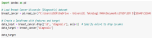
Fig. 1. Data Preparation Code

Training and Testing Dataset

Building an effective machine learning model involves dividing the dataset into training and testing sets. The training dataset, typically larger than the testing dataset, forms the foundation for the model’s learning process. Similar to the human brain, the model learns and discovers patterns from a substantial amount of data. The knowledge acquired during training is then evaluated using the testing dataset to measure the model’s accuracy in predicting results. This separation allows assessing how well the model generalizes to new, unseen data. The typical percentage of split training and testing datasets is 70% or 80% for training datasets and 30% or 20% for testing datasets.

However, in this study, to ensure robust evaluation with a limited dataset, 10-fold Cross-validation will be applied. This study applies a manual split method by creating a random column in the “breast_cancer.csv” files first. In that column, for every row generate a random number between 1 and 569 and sort the data using the “random” column. Delete the “random” column and this dataset is available for load. This process is essential to make sure that the dataset that will be divided into every fold is not biased, which means it will have a random total of benign and malignant data, instead of majoring in one case only (benign or malignant).

This dataset will then be subdivided into 10 folds, where each fold will have 56 to 57 data. The 10-fold Cross-validation approach enables a more comprehensive assessment of model generalization by iteratively using different partitions of the dataset for training and testing. For example, in fold 1, the first 57 data are used for the testing dataset and the rest would be the training dataset. It is important to note that all instances in the dataset will indirectly serve as training and testing datasets through this 10-fold Cross-validation process. Figure 2 shows the code for split training and testing datasets for every fold.

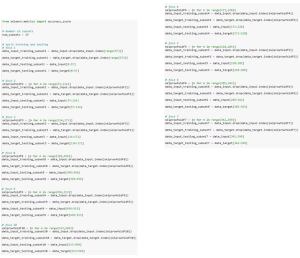
Fig. 2. Split Training and Testing Datasets Code

METHODOLOGY

In this study, three algorithms will be utilized to classify breast tissue as either benign or malignant. The overall flowchart in Figure 3 illustrates the entire process. As depicted in Figure 3, the construction of a machine-learning model for breast cancer prediction begins by loading the dataset and initializing the input features and target variables. Following this, the number of folds is set to ten. Subsequently, the data undergoes a split process into training and testing datasets for each fold by initializing the range of the data.

The cross-validation, SVM, RF, and KNN model functions are then initialized. Each algorithm’s function is called, where, within each algorithm’s function, the respective model is declared. In the case of the SVM, RF, and KNN models function, the cross-validation model function is invoked for training, making predictions, and calculating accuracy scores for each fold. The accuracy score calculation equation utilized is represented as:

Here,  is the number of folds while ​ is the model’s accuracy on the -th fold.

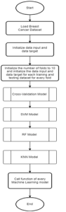
Fig. 3. Overall Flowchart

The three algorithms utilized in this study are as follows:

Support Vector Machine (SVM)

SVM is a supervised machine learning algorithm primarily used for classification problems usually referred to as a Support Vector Classifier (SVC) [12]. In SVM, each data point is represented as a point in an n-dimensional space, where n is the number of features. Classification is achieved by identifying the hyperplane that best separates different classes [12]. The equation of the hyperplane is represented as:

f(x)=w.x+b                                        (3)

Here,  is the weight vector,  is the input data, and  is the bias term.

SVM is particularly effective in high-dimensional spaces, making it suitable for datasets with numerous features. The algorithm provides flexibility through various kernel functions, such as Linear, Polynomial, Radial Basis Function (RBF), and Sigmoid, each serving different purposes. The Linear kernel is used for linearly separable data, while the RBF kernel captures complex relationships. The polynomial kernel introduces non-linearity to the decision boundary and the Sigmoid kernel is often employed for binary classification problems. To conclude, SVM aims to find the hyperplane with the maximum margin, contributing to its robustness in classification tasks.

Figure 4 illustrates the flowchart depicting the SVM model function. Within this function, each kernel of the SVM is explicitly declared. For every kernel variant, the cross-validation model function is invoked to both train and evaluate the model, subsequently returning the accuracy score. The resulting accuracy score from this function call is further computed by dividing it by the number of folds, which is set to 10. Finally, the resulting accuracy score is displayed. These accuracy scores will be compared to each other to select the best kernel for the SVM model. The best kernel is then chosen to be compared with the other algorithms.

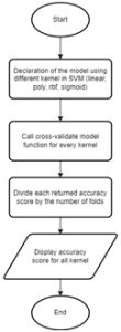
Fig. 4. SVM Model Function Flowchart

Figure 5 shows the code for the SVM Model function.

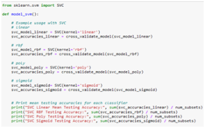
Fig. 5 SVM Model Function Code

Figure 6 shows the flowchart of the cross-validate model function. From Figure 6, the function of cross-validation is started by initializing an empty list to store accuracy scores. Subsequently, it enters an iteration for the training and testing datasets for each fold. The training dataset is then used to train the SVM model with different kernels. Following the training phase, the model is evaluated using predictions on the testing dataset to calculate the accuracy score for a particular fold, and this score is stored in the list. At the end of the iteration, the function returns the list of accuracies.

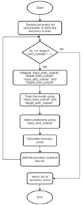
Fig. 6. Cross-Validate Model Function Flowchart

Figure 7 shows the code for the Cross-Validate Model function.

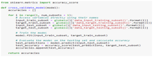
Fig.7. Cross-Validate Model Function Code

To build a machine learning model using this SVM model, it is necessary to invoke the SVM model function, as depicted in Figure 8, which illustrates the code for calling the function.

Fig.8. SVM Model Function Call Code

K-Nearest Neighbors (KNN) Algorithm

KNN is a straightforward yet powerful machine-learning algorithm designed for both classification and regression assignments. In KNN, predictions are determined by identifying the k-nearest neighbors of a given data point and determining the majority class or averaging the values of these neighbors [13]. The number of nearest neighbors can be manually set by initialization of the “n_neighbors” value. Increasing the number of neighbors generally improves the model’s performance up to a certain point, after which the benefits diminish. To conclude, KNN’s benefit lies in its simplicity and flexibility to adapt to various types of data, making it suitable for diverse classification tasks.

Figure 9 illustrates the flowchart depicting the KNN model function. Within this function, each number of nearest neighbors of the KNN is explicitly declared. For every number of nearest neighbors, the cross-validation model KNN function is invoked to both train and evaluate the model, subsequently returning the accuracy score. The resulting accuracy score from this function call is further computed by dividing it by the number of folds, which is set to 10. Finally, the resulting accuracy score is displayed. These accuracy scores will be compared to each other to select the best number of nearest neighbors for the KNN model. The best number of nearest neighbors is then chosen to be compared with the other algorithms.

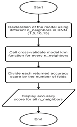
Fig. 9. KNN Model Function Flowchart

Figure 10 shows the code for the KNN Model function.

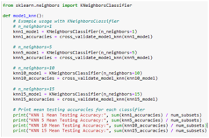
Fig. 10 KNN Model Function Code

The flowchart of the cross-validate model KNN function is the same as a cross-validate model function that is used by the SVM and RF models. Figure 12 shows the code for the Cross-Validate Model KNN function. The code is still the same as the Cross-Validate Model used by SVM and RF but some adjustments have been made in this function by adding “.to_numpy()” in this line of code as in Figure 11.

Fig. 11. Adjustments of Code in Cross-Validate Model KNN Model Function

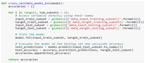
Fig.12. Cross-Validate Model KNN Function Code

To build a machine learning model using this KNN model, it is necessary to invoke the KNN model function, as depicted in Figure 13, which illustrates the code for calling the function.

Fig.13. KNN Model Function Call Code

Random Forest (RF) Algorithm

RF is a popular ensemble learning technique extensively employed in machine learning for tasks involving classification and regression. This study aims to use an RF Classifier to classify breast tissue by constructing a multitude of decision trees during training and outputs the mode of the classes (classification) [14]. The number of decision trees that be constructed can be manually set by initialization of the “n_estimators” value. Increasing the number of estimators generally improves the model’s performance up to a certain point, after which the benefits diminish. To conclude, RF excels in addressing overfitting, managing high-dimensional data, and delivering reliable predictions through the aggregation of outputs from numerous decision trees.

Figure 14 illustrates the flowchart depicting the RF model function. Within this function, each number of estimators of the RF is explicitly declared. For every number of estimators, the cross-validation model function is invoked to both train and evaluate the model, subsequently returning the accuracy score. The resulting accuracy score from this function call is further computed by dividing it by the number of folds, which is set to 10. Finally, the resulting accuracy score is displayed. These accuracy scores will be compared to each other to select the best estimators for the RF model. The best estimators are then chosen to be compared with the other algorithms.

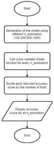
Fig. 14. RF Model Function Flowchart

Figure 15 shows the code for the RF Model function.

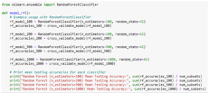
Fig. 15. RF Model Function Code

The cross-validation model function used by the RF model is the same as that used by the SVM Model. However, to build a machine learning model using this RF model, it is necessary to invoke the RF model function, as depicted in Figure 16, which illustrates the code for calling the function.

Fig.16. RF Model Function Call Code

RESULTS AND DISCUSSIONS

The results of applying the three classification models; SVM, KNN, and RF on the breast cancer dataset are shown in Table II, Table III, and Table IV, respectively. The model with the highest accuracy score will be chosen for each table, and the results will be summarized in Table V. This table will serve for further comparison between different models.

Results

Table 2 Accuracy Score Of The Svm Model

Kernels	Accuracy Score
Linear	95.61%
Poly	91.03%
RBF	91.73%
Sigmoid	45.01%

Based on the results in Table II, the results show that the Linear kernel produces the best accuracy score compared to other kernels. Thus, the Linear kernel is chosen to be compared with the KNN and RF model.

Table 3 Accuracy Score Of Knn Model

Number of Nearest Neighbors	Accuracy Score
1	91.04%
5	93.15%
10	92.79%
15	92.79%

Based on the results in Table III, the results show that the KNN with five as the number of nearest neighbors produces the best accuracy score compared to other numbers of nearest neighbors. Thus, the KNN with five as the number of nearest neighbors is chosen to be compared with the SVM and RF model.

Table 4 Accuracy Score Of Rf Model

Number of Estimators	Accuracy Score
100	95.96%
200	95.96%
500	96.31%
1000	96.31%

Based on the results in Table IV, the results show that the RF with 500 and 1000 as the number of estimators produces the best accuracy score compared to other numbers of estimators. Thus, the RF with 500 and 1000 as the number of estimators is chosen to be compared with the SVM and KNN models.

Table 4 Accuracy Score Of Each Model

Model	Remark	Accuracy Score
SVM	Linear Kernel	95.61%
KNN	5 as n_neighbors	93.15%
RF	500 and 1000 as n_estimators	96.31%

Based on Table V, the results show that the RF that used 500 and 1000 as the number of estimators produced the best accuracy score compared to other models.

Discussion

In this study, SVM, KNN, and RF are chosen as the three main algorithms in building the model for the prediction of breast cancer. Every algorithm has unique abilities that make it the best use for this prediction. The SVM model is known as the best model for classification tasks due to its versatility that are suitable for a variety of data [20]. In comparison, KNN is suitable as a classifier for breast cancer due to its adaptability. KNN operates by considering the majority class among the k-nearest neighbors, providing an intuitive and flexible decision-making process [22]. The simplicity of KNN allows for easy interpretation, as predictions are based on the similarities between instances in the feature space. The related studies also have shown that the KNN is also able to generate a good accuracy score in predicting breast cancer.

The RF model is selected due to its utilization of the combined outputs from multiple decision trees, which diminishes the impact of noise, resulting in improved outcomes [21]. This approach aids in controlling overfitting, consequently enhancing predictive accuracy. Moreover, the related studies have employed RF as the model for classifying the identical breast cancer dataset, consistently demonstrating commendable accuracy scores.

For the results, the RF model with 500 and 1000 as the number of estimators, outperforms SVM and KNN with an accuracy of 96.31%, compared to SVM with Linear kernel (95.61%), and KNN with 5 number of neighbors (93.15%). SVM’s slightly lower accuracy score may be attributed to its sensitivity to kernel choice and susceptibility to outliers. On the other hand, KNN’s reliance on local neighbors can make it less robust in the presence of noisy data. In contrast, RF’s ensemble learning, adeptness in handling high-dimensional data, and mitigating irrelevant features establish its superiority for achieving robust and accurate results in this context.

CONCLUSIONS

Based on Table V, the RF with 500 and 1000 as the number of estimators is the best model in predicting breast cancer as benign or malignant with a 96.31% accuracy score, while the KNN is the worst model. Thus, the RF with 500 and 1000 as the number of estimators is selected as the best model for the classification of breast cancer in this study. However, this model is suggested to be used primarily for medical diagnosis, particularly in the field of breast cancer detection.

REFERENCES

1. S. Kamarudin, I. Taib, I. Syafinaz, A. M. T. Arifin, and M. N. Abdullah, “Analysis of Heat Propagation on Difference Size of Malignant Tumor,” Journal of Advanced Research in Applied Sciences and Engineering Technology, vol. 28, no. 2, pp. 211–221, Oct. 2022, doi: 10.37934/araset.28.2.211221.
2. Saha, S. Banik, N. Mukherjee, T. Kanti, and D. Hod, “ASSOCIATION OF ABO BLOOD GROUP AND BREAST CARCINOMA AMONG CASES ATTENDING A TERTIARY CARE HOSPITAL, KOLKATA”, doi: 10.36106/ijsr.
3. Botticelli et al., “Positive impact of elastography in breast cancer diagnosis: an institutional experience,” J Ultrasound, vol. 18, no. 4, pp. 321–327, 2015, doi: 10.1007/s40477-015-0177-y.
4. Román et al., “Long-Term Risk of Breast Cancer after Diagnosis of Benign Breast Disease by Screening Mammography,” Int J Environ Res Public Health, vol. 19, no. 5, Mar. 2022, doi: 10.3390/ijerph19052625.
5. Bilal, A. Imran, T. I. Baig, X. Liu, E. Abouel Nasr, and H. Long, “Breast cancer diagnosis using support vector machine optimized by improved quantum inspired grey wolf optimization,” Sci Rep, vol. 14, no. 1, p. 10714, 2024, doi: 10.1038/s41598-024-61322-w.
6. Chen and Y. Jia, “Support Vector Machine Based Diagnosis of Breast Cancer,” in 2020 International Conference on Communications, Information System and Computer Engineering (CISCE), 2020, pp. 321–325. doi: 10.1109/CISCE50729.2020.00071.
7. Ghose, M. A. Uddin, M. M. Islam, M. Islam, and U. K. Acharjee, “A Breast Cancer Detection Model using a Tuned SVM Classifier,” in 2022 25th International Conference on Computer and Information Technology (ICCIT), 2022, pp. 102–107. doi: 10.1109/ICCIT57492.2022.10055054.
8. A. Aswathy and M. Jagannath, “An SVM approach towards breast cancer classification from H&E-stained histopathology images based on integrated features,” Med Biol Eng Comput, vol. 59, no. 9, pp. 1773–1783, 2021, doi: 10.1007/s11517-021-02403-0.
9. Telalović Hasić and A. Salković, “Breast Cancer Classification Using Support Vector Machines (SVM),” in Advanced Technologies, Systems, and Applications VIII, N. Ademović, J. Kevrić, and Z. Akšamija, Eds., Cham: Springer Nature Switzerland, 2023, pp. 195–205.
10. K. A. Enriko, M. Melinda, A. C. Sulyani, and I. G. B. Astawa, “Breast cancer recurrence prediction system using k-nearest neighbor, naïve-bayes, and support vector machine algorithm,” JURNAL INFOTEL, vol. 13, no. 4, pp. 185–188, Dec. 2021, doi: 10.20895/infotel.v13i4.692.
11. R. Sannasi Chakravarthy, N. Bharanidharan, and H. Rajaguru, “Deep Learning-Based Metaheuristic Weighted K-Nearest Neighbor Algorithm for the Severity Classification of Breast Cancer,” IRBM, vol. 44, no. 3, p. 100749, 2023, doi: https://doi.org/10.1016/j.irbm.2022.100749.
12. Cherif, “Optimization of K-NN algorithm by clustering and reliability coefficients: application to breast-cancer diagnosis,” Procedia Comput Sci, vol. 127, pp. 293–299, 2018, doi: https://doi.org/10.1016/j.procs.2018.01.125.
13. R. Al-Hadidi, A. Alarabeyyat, and M. Alhanahnah, “Breast Cancer Detection Using K-Nearest Neighbor Machine Learning Algorithm,” in 2016 9th International Conference on Developments in eSystems Engineering (DeSE), 2016, pp. 35–39. doi: 10.1109/DeSE.2016.8.
14. Chatakondu and K. Zhai, “An Analysis of the k-Nearest Neighbor Classifier to Predict Benign and Malignant Breast Cancer Tumors,” Journal of Student Research, vol. 12, no. 4, Nov. 2023, doi: 10.47611/jsrhs.v12i4.5577.
15. Minnoor and V. Baths, “Diagnosis of Breast Cancer Using Random Forests,” in Procedia Computer Science, Elsevier B.V., 2022, pp. 429–437. doi: 10.1016/j.procs.2023.01.025.
16. Dai, R.-C. Chen, S.-Z. Zhu, and W.-W. Zhang, “Using Random Forest Algorithm for Breast Cancer Diagnosis,” in 2018 International Symposium on Computer, Consumer and Control (IS3C), 2018, pp. 449–452. doi: 10.1109/IS3C.2018.00119.
17. A. Hasan Dalfi, S. Chaabouni, and A. Fakhfakh, “Breast Cancer Detection Using Random Forest Supported by Feature Selection,” International Journal of Intelligent Systems and Applications in Engineering, vol. 12, no. 2s, pp. 223–238, Oct. 2023, [Online]. Available: https://ijisae.org/index.php/IJISAE/article/view/3575
18. Batool and Y.-C. Byun, “Breast Cancer Classification using Random Forest Algorithm,” J Phys Conf Ser, vol. 2559, no. 1, p. 012002, 2023, doi: 10.1088/1742-6596/2559/1/012002.
19. S. Chudhey, M. Goel, and M. Singh, “Breast Cancer Classification with Random Forest Classifier with Feature Decomposition Using Principal Component Analysis,” in Advances in Data and Information Sciences, S. Tiwari, M. C. Trivedi, M. L. Kolhe, K. K. Mishra, and B. K. Singh, Eds., Singapore: Springer Singapore, 2022, pp. 111–120.
20. J. Smola and B. Schölkopf, “A tutorial on support vector regression,” Stat Comput, vol. 14, no. 3, pp. 199–222, 2004, doi: 10.1023/B:STCO.0000035301.49549.88.
21. Probst, M. N. Wright, and A.-L. Boulesteix, “Hyperparameters and tuning strategies for random forest,” WIREs Data Mining and Knowledge Discovery, vol. 9, no. 3, p. e1301, May 2019, doi: https://doi.org/10.1002/widm.1301.
22. Moeini, A. Shojaeizadeh, and M. Geza, “Supervised machine learning for estimation of total suspended solids in urban watersheds,” Water (Switzerland), vol. 13, no. 2, Jan. 2021, doi: 10.3390/w13020147.