
Sociodemographic Characteristics Mediated by Poverty as Determinants of Homeownership in Indonesia.
- Muhammad Saleh Mire
- 1018-1033
- May 23, 2024
- Economic Development
Sociodemographic Characteristics Mediated by Poverty as Determinants of Homeownership in Indonesia.
Muhammad Saleh Mire
Mulawarman University
DOI: https://doi.org/10.51244/IJRSI.2024.1104073
Received: 07 April 2024; Revised: 22 April 2024; Accepted: 26 April 2024; Published: 23 May 2024
ABSTRACT
This research focuses on homeownership status with antecedent variables of sociodemographic characteristics mediated by poverty, using panel data in 34 provinces in Indonesia during 2017-2023. This research uses a Path Analysis model with dummy variables, grouping regions into 2 groups, namely urban areas and rural areas. The research results show that GDP per capita and education have a significant negative effect on poverty both in urban and rural areas. Furthermore, family members and population density have a significant negative effect on poverty in both areas. Meanwhile, labor has no effect on poverty in the two regions as well as on homeownership in the city, but has a positive effect in rural areas. It was also found that male heads of household had a significant negative effect on poverty in urban areas but had no effect in rural areas, then poverty had a significant negative effect on house ownership in urban areas but had no effect in rural areas. Apart from that, education has no effect on homeownership in both urban and rural areas. Furthermore, homeownership is significantly influenced by population density and male head of household in rural areas but not significantly in urban areas.Increasing the ability to own a home can be done by alleviating poverty by providing cheap credit facilities to families who need a place to live. Furthermore, the government should pay attention to sociodemographic characteristicsin increasing people’s ability to own a home and it is hoped that there will be a follow-up with gender research on homeownership.
Keywords: GDP per capita, labor, population density, family members, male head of family, poverty and homeownership
INTRODUCTION
One of the most basic human needs is shelter, in addition to food, so humans try to fulfill it in conditions that vary according to their abilities and attractiveness or tastes. Housing is one of the most important components in the theory of urban economics which can be the most important part in measuring the welfare of society in general. The house is a place to unwind, a place to socialize and foster a sense of kinship among family members, a place for the family to shelter and store valuables, and also as a social symbol of status, therefore safety, liveability and environmental quality determine the choice in homeownership (Natalia, V. V. and Wunas, S., 2016). A house is considered a basic need that functions as a place to live or shelter and a means of family development. However, not all people or families can own a house with their own ownership status, because the costs of building and maintaining it are not easy to meet, especially in urban areas. Furthermore, if it is possible to make it happen, the issue of location is one of the considerations because the closer to the center the land or residence is, the more expensive it is, as explained by several location theories such as Weber’s theory and Christaller’s central place theory. Urban settlements increasingly have dilemmas due to migration from villages which will cause social and economic problems in urban areas (Todaro, and Smith, 2020).
Housing is often seen as a barometer of economic conditions. In recent years, policymakers and political leaders at local and national levels have begun to make stronger links between housing development and the economy at the local level and that is welcome. This new focus stems from the Lyons review report which emphasized the establishment of local government roles to promote economic prosperity and community well-being. The type and quality of housing offerings can have a significant impact on the health and wealth of a place. Their ability to attract and sustain themselves and provide support to those who need it depends on good housing and an attractive environment (Glossop, 2008).
Providing adequate housing or accommodation should be the responsibility of the state or government towards its people, as reflected in the Preamble to the 1945 Constitution and then explained in Article 28H paragraph (1) of the 1945 Constitution and in Article 40 of Law no. 39 of 1999 concerning Human Rights. To fulfill its responsibilities and realize the government’s commitment to providing services, the Indonesian government through the Ministry of Public Works and Public Housing has distributed Housing Financing Liquidity Facilities (FLPP) through the Center for Housing Financing Fund Management (PPDPP) since 2010 and carried out housing development activities which constitute the One Million Program Homes began to be implemented in 2015 (Ministry of PUPR: 2020) and explains that the 2021 One Million Houses program consists of 826,500 low-income (MBR) housing units and 279,207 non-MBR housing units. The details of the achievement of MBR houses consist of the results of house construction carried out by the Ministry of PUPR totaling 341,868 units, other Ministries/Institutions 3,080 units, regional government 43,933 units, housing developers 419,745 units, CSR Housing 2,270 units and the community 15,604 units.
Based on Law No. 4 of 1992 concerning Housing and Settlements, housing is a group of houses that function as residences or residential environments that are equipped with environmental facilities and infrastructure. Home is one of the basic needs of humans. Apart from food and clothing, a house as a place to live is one of the basic needs. Based on the Central Statistics Agency, the results of the Population Census (2020) in September 2020 recorded a population of 270.20 million people. The population from the 2020 Census increased by 32.56 million people compared to 2010 results. With Indonesia’s land area of 1.9 million km2, Indonesia’s population density is 141 people per km2. Meanwhile, the annual population growth rate during 2010-2020 averaged 1.25 percent, slowing down compared to the 2000-2010 period which amounted to 1.49 percent. This population increase has an impact on increasing demand for residential homes. On the other hand, according to (Citra Baskoro and Sartika Djamaluddin, 2023), the percentage of house ownership among households in Indonesia shows a decreasing trend from year to year. Limited supply of housing and high housing prices mean that most households use credit schemes to be able to own a home. This is contrary to data in research which shows a positive trend for homeownership in Indonesia, both in urban areas and villages. So homeownership is growing in the same direction as population growth, Figure 1.
Homeownership is largely determined by social, economic and demographic factors so that not all families can own a house to live in, in fact some city residents are more interested in renting a house than buying or owning their own, even if they have the ability. The rate of homeownership is higher in the Eastern Indonesia region compared to the Urban areas region, this is because the unemployment rate in the Urban areas region is also higher than the Eastern Indonesia region. Even though it is supported by the average disbursement of residential property credit which is higher in the Urban areas Region than the average disbursement of residential property credit in the Eastern Indonesia Region, this does not mean that the average level of homeownership in the Urban areas Region is also higher, this may be hampered with a lower average income and a higher average property price in the Urban areas Region than the Eastern Indonesia Region, so the risk of default is also higher in the Urban areas Region which can eliminate the ownership rights of a house purchased through a mortgage (Terate Sari and Wiguna, 2022).
Based on Figure 1, the homeownership rate from year to year shows a slightly upward trend with an average increase of only 1.63% for urban areas and 2.23% for rural areas, on the other hand, the population or number of families continues to increase. BPS noted that population growth reached 1.13%. So, if we compare the percentage increase in house ownership, it can be seen that in both urban areas and villages, the average increase in house ownership has exceeded population growth in both urban and rural areas. Based on the 2019 Bank Indonesia Residential Property Price Survey report, residential property sales in the first quarter of 2019 grew by 23.77% compared to the previous quarter. This growth increased compared to the previous quarter which experienced a decline of 5.78% and was also higher than the growth in the first quarter of 2018 which only grew 10.55%. Sales of residences in the small type house category have increased significantly. In the fourth quarter of 2018 there was a decline of 12.28%, but managed to increase in the first quarter of 2019 to 30.13%. The same thing also happened to the large house type, where in the fourth quarter of 2018 it decreased by 24.16%, but in the first quarter of 2019 it increased by 24.56%. Meanwhile, growth for medium-sized houses tends to slow down from 13.46% in the fourth quarter of 2018 to 13.33% in the first quarter of 2019. The improvement in sales was triggered by increasing sales of small and large house types. Apart from that, the stable growth in sales of large type houses also has a positive influence on residential property sales figures.
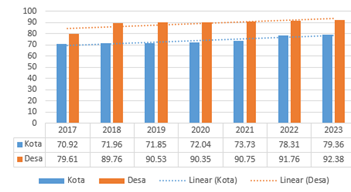
Figure 1. Development of Homeownership Percentage
The Central Statistics Agency (BPS) noted that the average provincial minimum wage (UMP) increased by 63.07%. If the average UMP is compared with the increase in house prices, it can be seen that house prices are higher compared to people’s income levels, in other words, house prices are currently above people’s purchasing power (unaffordable). Apart from purchasing power, the availability of infrastructure is also a challenge in providing public housing. The current real situation is that the Urban areas Region is seen as enjoying more development results than the Eastern Indonesia Region, this can be seen, among other things, from the proportion of regional contributions to the national Gross Domestic Product (GDP). According to data from BPS, in 2019 the Western Region of Indonesia contributed around 80% of the total National GDP, while the Eastern Region of Indonesia only contributed around 20%. Inequality in people’s living standards, especially in terms of economics and income, is one of the factors in the differences in access between regions in Indonesia to housing or housing, supported by other factors, namely the area and unequal distribution of the population. As in 2019, based on the publication of the Central Statistics Agency (BPS), Java Island with an area of 129,442 km² or only 6.74% of the total land area in Indonesia has a population of 150,408 thousand people, this number represents 56.35% of the total population. Indonesia, it can be said that the population density on the island of Java reaches 1,162 people/Km2. This density is much denser than Indonesia, which only has a density of 140 people/km. In addition, around 58.84% of the total number of households in Indonesia live on the island of Java, with high density causing limited land for residences or houses. Another obstacle faced by the government in providing public housing comes from an unproductive labor market which creates and exacerbates poverty.
The Central Statistics Agency recorded that the percentage of poor people in March 2023 was 9.36 percent, a decrease of 0.21 percentage points compared to September 2022 and a decrease of 0.18 percentage points compared to March 2022. The number of poor people in March 2023 was 25.90 million people, a decrease 0.46 million people in September 2022 and a decrease of 0.26 million people in March 2022. It was further stated that the percentage of urban poor people in March 2023 was 7.29 percent, a decrease compared to September 2022 which was 7.53 percent. Meanwhile, the percentage of poor rural residents in March 2023 was 12.22 percent, a decrease compared to September 2022 which was 12.36 percent. Compared to September 2022, the number of poor urban residents in March 2023 decreased by 0.24 million people (from 11.98 million people in September 2022 to 11.74 million people in March 2023). Meanwhile, in the same period, the number of poor rural residents decreased by 0.22 million people (from 14.38 million people in September 2022 to 14.16 million people in March 2023). In general, the poverty level in Indonesia has decreased from year to year. In 2012 poverty in Indonesia was 29.25 million. Then, it decreased in 2013 to 28.17 million. However, it experienced an increase in 2014 and 2015 with amounts of 28.28 million and 28.59 million. In 2016, it decreased again to 28.01. In 2017-2019, it continued to decline successively, namely 27.77 million; 25.95 million; and 25.14 million or 9.14%. Furthermore, the poverty rate as of March 2022 has decreased again to 9.54%, from 9.71% in 2021 and in 2023 it will decrease again to 9.36%, Figure 2.
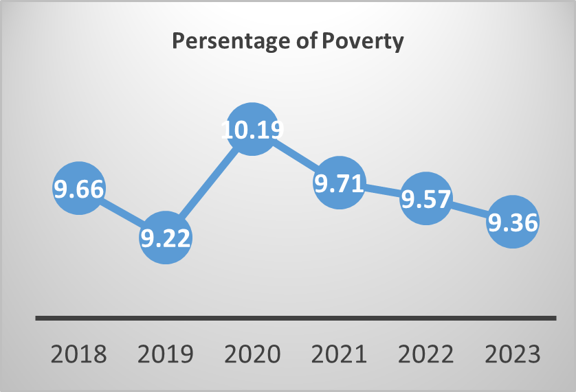
Figure 2. Development of Poverty Percentage
One of the social factors that influence homeownership is education. It is hoped that as a person’s education increases, the population’s opportunity to meet their housing needs can be achieved both directly and indirectly through income level. Furthermore, at a macro level, per capita income can influence or determine a person’s ability to own a house. Apart from education level, homeownership can also be determined using demographic factors such as population density, number of family members, and the percentage of male heads of families in the population. The relationship between sociodemographic factors and homeownership which is mediated by poverty can be seen in Figure 3.
RESEARCH OBJECTIVES
This research aims to analyze and examine the effect of sociodemographic characteristics on poverty and homeownership in the form of:
- Compare the relationship between sociodemographic factors and homeownership of the two regions
- Assess the effect of population density, family members, GDP per capita, the percentage of male heads of families, labor, education, and poverty on homeownership
- Examining the effect of GDP per capita, population density, family members, the percentage of male heads of families, education and labor on poverty
- Assess the total effect of sociodemographic factors on homeownership
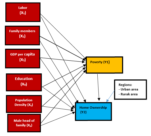
Figure 3. Framework
LITERATURE REVIEW
Homeownership Level Homeownership Level can be seen from the percentage of ownership status of a residence or owned house (Buhaerah, 2019). In Germany, homeownership is a housing unit that is legally owned by an individual or household and is used as a residence or wealth asset (Bentzien et al., 2012). Homeownership is influenced by several determinants, namely relative costs such as rental costs, credit interest and so on, credit restrictions, house prices, government policies and geographical location (Bourassa et al., 2015). Other findings state that homeownership is influenced by several determinants, namely relative costs such as rental costs, credit interest, and so on, credit restrictions, house prices, government policies and geographical location (Bourassa et al., 2015). Furthermore, Sari and Wibowo, 2012 examined house ownership which was influenced by 4 independent variables: residential property credit, income, and unemployment, it was found that income and unemployment had a significant influence on ownership. Furthermore, income has a negative relationship with the level of homeownership in 3 models, namely Indonesia, the Urban areas Region, and the Eastern Indonesian Region, which means that every increase in income and unemployment rate will have an effect on decreasing the level of Homeownership in Indonesia, the Urban areas n Region and the Eastern Indonesian Region. This is supported by the results of previous research which states that income will affect people’s purchasing power if the increase in house prices is not proportional to the increase in household income, it will make house prices remain unaffordable for households because house prices are still above household purchasing power even though an increase in income and increasing unemployment will make obstacles in accessing the mortgage market greater and increase the risk of default due to the increasing uncertainty of household income (Sari and Wiguna, 2022).
According to Blanco et al. (2014), there is a relationship between income and household ownership of a house. When household income is low, the household’s decision to rent a house will be a better choice than owning housing even with a mortgage (Blanco et al., 2014). This opinion is supported by research conducted by Botello (2020) Homeownership Rate in Columbia, among the results of which are Columbia residents, especially young people with low and middle incomes, tend to prefer rental housing compared to buying a house, this makes income one of the factors determining the level of homeownership in Columbia in addition to home prices and variations in housing development areas (Botello-Peñaloza, 2020). Income, which is one of the financial constraints of households, has a negative correlation with the level of homeownership, this is because households with low incomes will be vulnerable to financial restrictions such as loan restrictions or amortization requirements (Enstrom-Ost et al., 2017).
The housing market, which can describe the economic capacity of a household, is an important factor in determining ownership, when labor market performance is low so that the unemployment rate increases, affected households will lose their economic capacity due to reduced income which also reduces ownership in the housing market. (Doling et al., 2015). Income is obtained from the sacrifice of labor services, more and more of the workforce will work and earn income so that they can have stable finances which will then make it easier to access the housing mortgage market (Desy Delvina Wijaya & Anastasia, 2021). A high cost of living will impact the cost of salary increases and business rent levels, as well as impact business location and expansion decisions. House price inflation can also provide collateral for new businesses. A region where house prices rise in real terms will become richer and may invest some of the wealth in new companies. In areas with lower levels of demand but a limited range of housing services are often limited to attracting the necessary workers and limiting growth. The housing system can also be an important economic sector in terms of capital employed, employment directly from construction, sales and turnover, and repair and maintenance of housing. Basically, homeownership is also influenced by the level of education, because expenditure includes consumption, so it is in accordance with Keynes’ theory (Branson, William H. 1992).
Humans are creatures who are always involved in the educational process, whether carried out on other people or themselves. The educational process is a universal activity in human life, because wherever and whenever in the world there is education. Even though education is a common phenomenon in every society, the differences in philosophy and outlook on life adopted by each nation or society and even individuals cause differences in the implementation of these educational activities. Thus, apart from being universal, education is also national. Its national character will color the nation’s education. According to Law no. 20 of 2003 Education is a conscious and planned effort to create a learning atmosphere and learning process so that students actively develop their potential to have religious spiritual strength, self-control, personality, intelligence, noble morals, and the skills needed by themselves, society, nation, and country. The causal relationship between education and economic growth is becoming increasingly proven and strong; 2) the education sector as the main driver of the dynamics of economic development increasingly encourages long-term structural transformation processes, because education provides a high rate of return in the future (Robelo, 1949). Furthermore, lack of socio-economic access, especially income, is directly related to poverty.
The concept of poverty is multidimensional. Sida divides poverty into 4 dimensions, namely: Resources, power and voice, opportunity and choice, and human security. So theproblem of poverty is not only in the form of material fraud but also in other dimensions.Furthermore, Adisasmita (2006: 144) states that the indicators of poverty in rural communities are: (1) lack of opportunity to obtain education, (2) having limited agricultural land and capital, (3) no opportunity to enjoy investment in the agricultural sector, (4) no fulfillment of one of the basic needs (food, shelter, housing, (5) using traditional agricultural methods, (6) lack of business productivity, (7) no savings, (8) poor health, (9) no insurance and social security, (10) the occurrence of corruption, collusion and nepotism in village government, (11) not having access to clean water, and finally (12) lack of participation in public decision making.
Poor people do not have sufficient income and consumption to lift them from the minimum adequate level. So in short, poor people are those who live below the poverty line, which is determined by a national or international institution. So understanding of poverty covers not only economics, but has expanded to cover various aspects of life, including other social dimensions, such as health, and education and even entering the political dimension. However, the definition of poverty is the inability to meet minimum standards of needs, both food and non-food. This kind of poverty is also called absolute poverty, contrastedwith relative poverty. Apart from that, Indonesia is known for structural poverty and temporary poverty. Structural poverty is certainly worse than temporary poverty because, in this type of poverty, it is difficult to get out of poverty. After all, it has become chronic (chronic poverty) which is characterized by deprivation, discrimination, and living in areas that do not support the improvement of life.
THE METHOD
This type of research is quantitative, taking the type of study of comparative causality that processes numerical data that can be calculated using statistical formulas. The data analysis technique used in this study is path analysis which estimates the direct and indirect influence of exogenous variables on endogenous variables although in this study we only look at and discuss the direct effect, both effects are available in the statistical program used for estimation in this study. This study uses secondary data, namely data that is already available and collected by other parties and it was panel data. The data was taken from the Indonesia Central Statistics Agency (BPS) and the Ministry of Public Works and Public Housing (PUR) which covers 34 provinces in Indonesia, where since the end of 2022 there have been 38 provinces, but the necessary data is not yet available. The data used is divided into two groups, Region 1 and Region 2. The statistical analysis technique used is path analysis using the Amos 18 statistical application program.
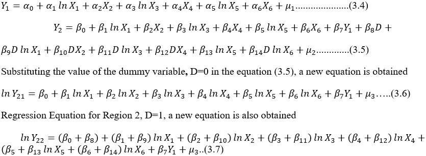
Based on the conceptual relationship in the framework of thinking, mathematically functional relationships can be written as
Y1= f(X1, X2, X3, X4,X5, X6)
Y2= f(X1,X2, X3, Y4, X5, X6, Y1, D, DX1, DX2, DX3, DX4,DX5, DX6)
Whereas:
X1 = labor (number of employed workforce)
X2 = family members (percentage offamilies with 6 members and above)
X3 = GDP per capita (national production at constant prices divided by population)
X4 = education (average length of time the population has attended formal education, year)
X5 = population density (ratio of the population to area of a province)
X6 = male head of family (percentage of male heads of families to the population)
Y1 = poverty (percentage of poor people to the total population)
Y2 = homeownership (percentage of family heads who own a house to the number of family heads)
D = Dummy variable, D = 0, Urban area (Region 1); D=1, Rural area (Region 2)
Based on the conceptual relationship in the framework of thinking, mathematically functional relationships can be written as
Based on the conceptual relationship in the framework of thinking, mathematically functional relationships can be written as
RESULTS AND DISCUSSION
Model fit test
Chi-square statistic, as stated earlier, is the most fundamental test to measure overall fit, it is very sensitive to the size of the sample used and the relation of exogenous variables, almost the same as the model Regresi Linear Berganda. The model is considered good if the Chi-square value is small. The smaller the value, the more feasible the research, meaning that the more it describes the match between the variance of the sample taken and the research population. The results of data processing that have been carried out using the AMOS 18 program are shown in Table 1.
Table 1. Goodness of Fit Index
| No. | Goodness of fit Measure | Cut-off Criteria | Estimation (cut off Value) | Fit Situation |
| 1 | Chi-Square (χ2 )
Significance Probability (p) |
smaller the better
≥0.05 |
2.536
0.804 |
Fit |
| 2 | RMSEA (the Root Mean Square Error of Approximation) | ≤ 0.05 | 0.000 | Fit |
| 3 | NFI (Normed of Fit Index) | ≥0.95 | 0.998 | Fit |
| 4 | IFI (Incremental Fit Indices) | ≥0.95 | 0.103 | Fit |
| 5 | CMIN/DF (the minimum Sample Discrepancy Function) | ≤ 2 | 0.423 | Fit |
| 6 | TLI (Tucker Lewis Index) | ≥0,95 | 1.928 | Fit |
| 7 | CFI (Comparative Fit Index) | ≥0,95 | 1.000 | Fit |
| 8 | Hoelter’s Index | ≥200 | 2018 | Fit |
Resource: Malkanthie, 2015; Wan, 2022 and Amos Result
Research findings
As is known, this research divides Indonesia’s provinces into 2 regions, so the estimation results consist of two components. The estimation results for Region 1, which is called urban area, D=0, can be seen in Figure 4.
 |
|

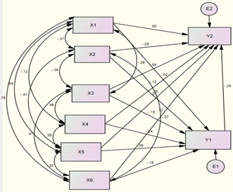
Figure 4. Coefficients of exogenous variable in Urban Areas and Result of Default Model
Recourse: Amos 18 data processing results.
As can be seen in Figure 2, where there is no level of confidence or probability for each coefficient or path, the estimation results are also displayed as a scalar estimate for Region 1 (Group 1), which describes the level of significance of each path, Figure 5.
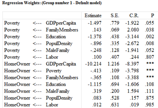
Figure 5. Scalar Estimates in Urban Areas
Resource: Amos 18 data processing results.
Further illustrating the estimation results for Region 2, named Rural Area, D=1, as carried out in Region 1, can be seen in Figure 6.
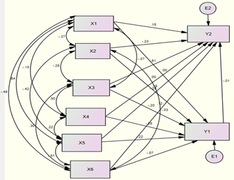
Figure 6. Variabel Coefficients in Region 2
Resource: Amos 18 data processing results
Next, in Region 2, the estimation results are presented, variable coefficients with confidence level or probability (P), RegressionWeights for Region 2, can be seen in Figure 7.
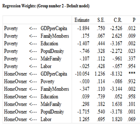
Figure 7. Scalar Estimates Region 2
Resource: Amos 18 data processing results
The results of the analysis show the influence of one variable on another variable according to the research objectives, based on Figure 3 and Figure 4, a summary of the influence of independent variables on dependent variables can be represented in Table 2. The table also shows that Region 1 (urban areas) and Region 2 ( rural areas) each have a coefficient and probability according to the relationship between variables. It also shows the total influence of sociodemographic variables consisting of: GDP per capita, family members, education, population density, male family, labor on poverty, and homeownership.
RESULTS AND DISCUSSIONS
The employment opportunities has no effect on poverty and homeownership in both rural and urban areas. This is because workers generally receive minimum wages, some even below the UMP, which is unable to lift people out of poverty. This is because the workforce works in MSMEs where more than 97% (the highest in the world) of people work in this sector (BPS, 2022). Almost the same or in a different context, the research conducted by (Purnomo and Kusreni, 2019) stated that employment opportunities had a positive influence on poverty in East Java, Indonesia. So if job opportunities increase it will cause an increase in the number of poor people.
GDP per capita has a significant negative effect on poverty both in urban and rural areas at a confidence level of α= 10% with regression coefficients of -1.49 and -1.894, meaning that if there is a 1% increase in GDP per capita, it will cause decreasing poverty 1.49 % in rural area and 1.845% in rural areas, assuming other independent variables are constant in the model. Furthermore, it is also known that this variable has a negative influence on homeownership. This fact supports the research of(Phang, 2013; Sari and Wibowo, 2022) which states that there is a correlation between the level of homeownership which is relevant to the level of income per capita in accessing mortgages for housing financing.
Furthermore, family members or the highest percentage of family members (6 people and above) have a positive effect on poverty. So if family members increase, poverty will worsen. This effectis significant for poverty at a confidence level of α= 5% with a regression coefficient of 0.14, meaning that every 1% increase in family members will have an impact on increasing poverty by 0.14%. The table also shows that the relationship between education and poverty is negative, meaning that if education increases then poverty decreases in the city, as has been shown in many studies (Mire at al., 2023). The same thing also happens in rural areas with a regression coefficient of -1.41, which means that if education increases by 1 year then poverty will decrease by 1.41% assuming other independent variables are constant in rural areas.
Table 2. Coefficients of the variables in Region 1 and Region 2,
| No | The Relation of the variables | Urban Areas | Rural Areas | ||||
| Dependent variables | Independent or exogenous variables | Coefficient | Probability | Coefficient | Probability | ||
| 1 | Unstandardized Direct Effect | Poverty | 1. GDP per Capita
2. Family Members 3. Education 4. Population Density 5. Male Family 6. Labor |
-1.497
0.143 -1.378 -0.896 -0.248 1.000 |
0.055
0.038 0.002 0.008 0.052 0.807 |
-1.894
0.175 -1.407 -0.746 -0.107 -0.025 |
0.012
0.009 0.002 0.023 0.337 0.945 |
| 2 | Homeownership | 1. GDP per Capita
2. Family Members 3. Education 4. Population Density 5. Male Family 6. Labor 7. Poverty |
-10.214
–0.365 -1.115 0.083 0.319 0.012 -0.413 |
0.000
0.000 0.108 0.875 0.111 0.985 0.000 |
-10.054
-0.347 0.039 -1.715 0.298 1.265 -0.010 |
0.000
0.002 0.958 0.001 0.101 0.069 0.932 |
|
| 3 | Standardized Total Effect | Poverty | 1. .GDP per Capita
2. Family Members 3. Education 4. Population Density 5. Male Family 6. Labor |
-0.153
-0.151 -0.245 -0.264 -0.151 0.020 |
-0.196
0.193 -0.250 -0.217 -0.074 -0.005 |
||
| 4 | Homeownership | 1. GDP per Capita
2. Family Members 3. Education 4. Population Density 5. Male Family 6. Labor 7. Poverty |
-.598
-0.285 -0.059 0.081 0.156 -0.004 -0.251 |
-0.613
-0.227 0.005 -0.293 0.122 0.152 -0.006 |
|||
Source: Data Processing Results, 2024.
Previous research conducted by Bramley, (Glem at al., 2007) stated that homeownership has an additional effect on school attainment, beyond that explained by poverty and other associated variables. However, research also shows that poverty can have a direct influence on homeownership. The results of this research show that there is a negative and significant direct effect of poverty on homeownership with a regression coefficient of -1.12% in the city. However, in rural areas, it has no effect. So this research finds that there is a reciprocal relationship between homeownership and poverty levels. One of the factors that can cause education to not have an influence on homeownership in rural areas is not due to the low percentage of homeownership compared to urban areas, but the main factor is that the fact shows that the average level of education in urban areas is higher than the level of education in rural areas (BPS, 2022), so it is natural that education does not have an influence on homeownership in rural areas.
Furthermore, population density has a significant negative influence at the confidence level α= 5% on poverty in the city. The population density in the city can be understood because the urban area in the city center is where rich people live or are generally inhabited so that almost no poor families are found. So it is natural that the influence of population density has a negative effect on poverty. This is different in rural areas where significant population concentrations are not found because very few people live in rural areas compared to urban areas, such as the Papua region which is inhabited by mostly poor people, but the density is low..
Furthermore, it can also be seen that the influence of the percentage of male heads of household in the family has a significant negative influence on poverty at the confidence level α= 5%. So the higher the percentage of heads of families, the lower the poverty level in the city. This fact shows that the male gender is still dominant in improving the family’s standard of living, believing it can reduce poverty rates. Men act as subjects, as main actors, and women as objects or extras (complements). Therefore, men act as the main breadwinners and women as additional breadwinners. Men as leaders in the family (Sri Suhandjati, 2017).
This male leadership as the main subject and actor in the family can work hard so that there is an increase in income which results in the percentage of poverty being reduced over time. In this way, homeownership can also increase. As research shows, poverty has a significant negative effect at the confidence level α= 10% in urban areas, but has no effect in rural areas. As a result, poverty has a significant negative effect in urban areas but has no effect in rural areas. If poverty can be reduced by 1% in the city, there will be an increase in homeownership in the city by 0.41%. According to the Central Statistics Agency, in 2023 the depth of poverty and severity with respective indices (1.163; 0.028) in urban areas will be lighter than in rural areas with indices (2.035; 0.511). This results in poverty being reduced more easily in urban areas than in rural areas, which has the implication that the negative influence of poverty on homeownership is significantly negative.
This research discusses the influence of sociodemographic factors on poverty and homeownership so that direct and indirect influences can be discussed in depth. Direct influence has been discussed, now we will discuss total effect (direct effect + indirect effect). From Table 2, the total influence can be seen, so it can be explained: The biggest total influence among the 6 exogenous variables is the influence of education on poverty both in urban areas and rural areas, while on house ownership, in the same table, it can be seen that there are seven variables that have an influence The total and largest is per capita income in both urban and urban areas. It’s just that the effect of total GDP per capita on homeownership is negative, this fact supports a direct effect. So the higher the per capita income, the lower the level of homeownership.
CONCLUSION AND RECOMMENDATION
Conclusion
Based on the analysis and the results of the previous discussion, the following conclusions are drawn:
- GDP per capita and education have a significant negative effect on poverty both in urban and rural areas
- The number of family members and population density have a significant negative effect on poverty both in urban and rural areas
- Labor has no effect on poverty in either urban or rural areas, nor does it have a positive effect on homeownership in urban areas, but has a positive effect in rural areas
- The percentage of male heads of household has a significant negative effect on poverty in the city. However, in rural areas, it has no effect
- Poverty has a significant negative effect on homeownership in urban areas, but in rural areas, it has no effect
- Education did not affect homeownership in both urban and rural areas
- Population density affects homeownership in rural areas, but not in urban areas
- Homeownership is significantly influenced by male heads of household in rural areas but not significantly in urban areas.
- The biggest influence of sociodemographic factors on homeownership is GDP per capita.
Recommendation
The suggestions to be put forward based on the discussion and conclusions that have been stated, among others:
- Poverty is still a major problem in development, therefore the government should increase GDP per capita through monetary and fiscal policies and always strive to improve the quality of human resources.
- One effort that can be made to improve the condition of homeownership is to eradicate poverty by providing cheap credit facilities to families who need a place to live.
- Socio-demographic factors should be the main concern in the government’s efforts to increase the population’s ability to own a home
- New research looks at the role of men’s leadership in the family in poverty alleviation and homeownership. It is hoped that there will be a follow-up with gender research on poverty and homeownership.
REFERENCE
- Adisasmita, R. (2006). Rural and Urban Development. Science House
- Branson, W. H. 1992. Macroeconomics Theory and Policy. Hopper & Row Publishers, Singapore.
- 2023. Gross Regional Domestic Product of Provinces in Indonesia According to Expenditure, 2018-2022. Jakarta
- 2023. Statistical Year Book of Indonesia. Catalog Number: 1101001, Publication Number: 03200.2303, ISSN/ISBN: 0126-2912, Jakarta.
- Blanco Blanco, Andrés & Fretes Cibils, Vicente & Muñoz Miranda, Andrés & Gilbert, Alan & Webb, Steven & Reese, Eduardo & Almansi, Florencia & Del Valle, Julieta & Pasternak, Suzana & Brain, Isabel & M, 2014. Rental Housing Wanted: Options for Expanding Housing Policy. IDB Publications (Books), Inter-American Development Bank, number 6730. https://publications.iadb.org/handle/113 19/6730
- Botello-Peñaloza, H. (2020). Homeownership Rate and Other House Price Determinants Impacts on New House Prices in Colombia. Journal for the Advancement of Developing Economies, 35–50. https://doi.org/10.32873/unl.dc.jade913
- Buhaerah, P. (2019). Kajian Ekonomi & Keuangan Pengaruh Kredit Pemilikan Rumah terhadap. Kajian Ekonomi Keuangan, 3(3), 182–197
- Bourassa, S. C., Haurin, D. R., Hendershott, P. H., & Hoesli, M. (2015). Determinants of the Homeownership Rate: An International Perspective. Journal of Housing Research, 24(2), 193–210. https://doi.org/10.1080/10835547.2015. 12092104Mankiw, Gregory. 2000. Macroeconomics. Worth Published, Harvard University. Ninth Edition. Macmillan Education Imprint. New York
- Bentzien, V., Rottke, N., & Zietz, J. (2012). Affordability and Germany’s low homeownership rate. International Journal of Housing Markets and Analysis, 5(3), 289–312. https://doi.org/10.1108/1753827121124 3616
- Citra Baskoro and Sartika Djamaluddin, 2023. The Effect of Income Uncertainty on Homeownership Status in Indonesia. Berdikari: Indonesian Journal of Economics and Statistics (JESI) Articles, Vol 3, No 2.
- Desy Delvina Wijaya and Anastasia, N. (2021). Millennial Generation Considerations on Homeownership. Journal of Asset Management And Valuation, pages 11–20.
- Doling, J., Karn, V., & Stafford, B. (2015). The Impact of Unemployment on Homeownership. Housing Studies, 1(1), 49–59. https://doi.org/10.1080/0267303860872 0562
- Enstrom-Ost, C., Söderberg, B., & Wilhelmsson, M. (2017). Homeownership rates of financially constrained households. Journal of European Real Estate Research, 10(2), 111–123. https://doi.org/10.1108/JERER-09- 2015-0035
- Glem, Bramley and Karley, N.K., 2007. Homeownership, Poverty and Educational Achievement: School Effects as Neighborhood Effects. Housing Studies, Volume 22, 2007 – Issue 5, Pages 693-721, https://doi.org/10.1080/02673030701474644.
- Glossop, G. (2008). Housing and Economic Development. Housing Corporation.
- Haughton, Jonathan. Khandker and Shahidur R. 2009. Handbook on Poverty and Inequality. The International Bank for Reconstruction and Development/The World Bank1818 H Street, NW.
- Law of the Republic of Indonesia Number 20 of 20023 concerning the National Education System. Jakarta.
- Malkanthie, Asoka. 2015. Structural Equation Modeling with AMOS Book. March 2015;DOI: 10.13140/RG.2.1.1960.4647
- Ministry of Public Works and Public Housing (PUPR), 2022. Jakarta SP.BIRKOM/I/2022/33
- Wan, T. T. H. (2002). Evidence-based health care management: Multivariate modeling approaches (1st ed.). Norwell, MA: Kluwer Academic Publishers.
- Natalia, Venny Veronica, and Wunas, Shirly. 2016. Housing Development: Signs and Symptoms in Middle Urban areas of Indonesia. ScienceDirect, Journal and Book. https://doi.org/10.1016/j.sbspro.2016.06.072.
- Phang, S. Y. (2013). Housing Finance Systems: Market failures and government failures. In Housing Finance Systems: Market Failures and Government Failures. https://doi.org/10.1057/9781137014030
- Purnomo, Agus Budi and Sri Kusreni. 2019. The Effect of Investment, GRDP and Workforce Matching on the Number of Poor People. Airlangga Journal of Economics and Business Volume 29, No.2, June – November 2019, p-ISSN: 2338-2686 e-ISSN: 2597-4564 Page 79 – 93
- PUPR: 2020. PUPR Ministry’s Subsidized Housing Assistance Program, Highest Achievement in 2021 FLPP Fund Distribution Since 2010
- Sari, K. T. & Wiguna, A. B. 2022.Homeownership Rates in Indonesia. Contemporary Studies in Economics, Finance, and Banking. Volume 01, Number 3, Pages 466-479. http://dx.doi.org/10.21776/csefb.2022.01.3.09
- Sida, 2017. Dimensions of Poverty Sida’s Conceptual Framework. Sitrus Art. no.: Sida 62028en urn:nbn:se:sida-62028en, ISBN: 978-91-586-4259-1
- Sri Suhandjati, 2017. Male Leadership in the Family: Its Implementation in Javanese Society Journal of Theologia, Vol 28 No 2 (2017), 329-350,ISSN 0853-3857 (print) – 2540-847X (online) DOI: http:/ /dx.doi.org/10.21580/teo.2017.28.2.1876
- The preamble to the 1945 Constitution and then explained in Article 28H paragraph (1) of the 1945 Constitution and in Article 40 of Law no. 39 of 1999 concerning Human Rights.
- Todaro, Michael P. and Smith, Stephen C. 2020. Economic Pearson, Addison-Wesley Boston Columbus Indianapolis New York San Francisco.
- Weiss, John, 2005. Poverty Targeting in Asia: Experiences from India, Indonesia, the Philippines, the People’s Republic of China, and Thailand. Asian Development Bank Institute, Tokyo.