Developing a Framework on Modeling Dependence across Stock Markets using Copulas: A Case of 5 SADC Stock Markets

Developing a Framework on Modeling Dependence across Stock Markets using Copulas: A Case of 5 SADC Stock Markets

Brian Basvi

University of Zimbabwe

DOI: https://doi.org/10.51244/IJRSI.2024.1105050

Received: 15 May 2024; Accepted: 27 May 2024; Published: 14 June 2024

ABSTRACT

Selecting the right dependence measure is crucial for multivariate statistical modelling. Because correlation is based on the elliptical distributions assumption of normalcy, which breaks down when there are extreme endpoints in either marginal or higher dimension, correlation is fraught with dangers. Copulas provide an alternate dependence measure that gets over correlation’s drawbacks and can be used to identify if a reliance is linear, upper tail, or lower tail. In order to evaluate the efficacy of regional integration, this study investigates whether copulas are suitable for simulating bivariate reliance among five SADC stock markets. The research design used in the study was explanatory and descriptive. Because of their favourable characteristics, Archimedean copulas were investigated using both parametric and non-parametric methods. Because the markets were likely to boom concurrently, non-parametric estimate produced insightful results demonstrating the suitability of the Gumbel copula in dependence modelling and suggesting that investors have opportunities for portfolio diversification throughout the region.

Key Words: Correlation, Copulas, Dependence, Multivariate statistical modelling

INTRODUCTION

The notion of interdependence among financial markets has been extensively researched since it is crucial for making decisions about risky assets and different types of economic platforms. Numerous techniques, including as factor analysis, principal component analysis, and regression, are available in multivariate analysis for the examination of dependence. The copula models, joint distributions, and conditional correlation calculation are the methods that are most frequently utilized. Unfortunately, for commodity price data, which are known to be leptokurtic, the normality assumption upon which it is based is negligible. The joint distributions option assumes a multivariate normal distribution on the majority of datasets. According to De Carlo (2021), measurements near the tails of the distribution actually have a greater impact on kurtosis than measurements in the centre of the distribution. It was claimed, as with earlier Hopkins (2020), that skewed data are invariably leptokurtic. As we attempt to align our data under consideration in respect to this consolidated literature the majority of which has been concluded on data from industrialized countries this raises curiosity in both the nature and extent of the measures of dispersion indicated by the data.

The main statistic in a joint normal distribution is the linear correlation coefficient, and Embrechts et al. (2022) highlighted the drawbacks and restrictions of applying it to the analysis of dependence. The linearity assumption has guided the majority of our investigation of associations, which has limited our ability to understand complex relationships in econometrics. Outside of elliptical distributions, which include the normal distribution and its mixing distributions, linear correlation is just a useful measure of reliance and can lead to a number of misconceptions. Count (2021) states that the distributional trait of heavy tails is exhibited by numerous commodity prices and financial time series, and for some heavy-tailed distributions, linear correlation is not specified. The alternate method for computing conditional correlations has a drawback in that the resulting correlations have been discovered to be inadequately informative when asymmetric dependency (correlation breakdown) exists, i.e., when stock index correlations have a tendency to rely on the direction of the markets, as predicted by Boyer, Gibson, and Loretan (2023).

Given how frequently transformations are employed in finance and economics, the copula model’s invariance under rising and continuous transformations is a helpful characteristic. Since the probability integral transformation plays a key role in the definition of copulas, it is confirmed that copulas are suited for studying dependence because they aid in explaining the degree of dependence regardless of the datasets’ distribution functions. Copulas are also employed in the definition of non-parametric measures of association, which are helpful in the parameter estimation of copula models. Examples of these measures are Kendall’s tau τ, Spearman’s rho ρ, and Schweizer and Wolff’s sigma σ. The copula can record tail dependence, which is a probability measure of the likelihood that the two variables under study are in their extremes, a crucial idea in a variety of financial applications. Copulas are extremely important for study in the domains of finance and economics since they take into account both the structure and the degree of dependence.

LITERATURE REVIEW

2.1 Application of Copula in Finance

In their working paper on risk management, Embrechts et al. (1999) used copula modelling of reliance for the first time in the finance industry. This idea has gained popularity in a variety of fields, including credit risk, time-varying dependency of multivariate time series, contagion, tail dependence, portfolio and market value-at-risk (VaR) computations, and multivariate option pricing. Because of the non-normal dependence, copula methods were used by Cherubini and Luciano (2001), to study the value-at-risk of portfolios. To ascertain the strong correlations between global equity markets, Longin and Solnik (2001) employed a Gumbel copula. Marshal and Zeevi (2002) estimated the degrees of freedom in a t copula to test the Gaussian assumption in financial markets. Pricing derivatives Cherubini et al. (2019) took into consideration the use of copulas because of the influence of non-normal dependence on trade and pricing.

Ling Hu (2021) summarized the reliance structure in various major stock markets using a mixed copula model, which captures all sorts of dependence levels. The model was composed of three copulas: Gaussian, Archimedean and Gumbel survival, the latter of which accommodated asymmetric tail dependency. A two-stage semi-parametric approach was used to estimate the model; this method is robust and free from some mistakes arising from the marginal distributions. The Maximum Likelihood technique was employed to estimate the parameters. The resulting model proved to be beneficial in constructing the joint distributions by applying Sklar’s Theorem. It was advised to first filter the empirical data because the presence of conditional heteroscedasticity in the financial data limited the importance of the model results.

 A phenomenon known as financial contagion best illustrated by the 1997 crash of the Asian markets occurs when difficulties in one market cause significant issues in other markets that are unexpected. By focusing on the levels and variations in dependency, Rodriguez (2005) provided the first application of copulas to contagion through the use of a Markov switching copula model. Bartram et al. (2016) investigated financial market integration amongst seventeen European stock market indexes using a time-varying conditional copula. Patton (2018) concentrated on using copulas with a temporal-variation allowance in financial time series applications. This resulted in an extension of Sklar’s Theorem to time series data, provided that all of the marginal distributions in the copula have similar information sets. He applied the method of Inference Function Model (IFM) which is divided into two parts: parameter estimation for the copula conditional on the estimates derived for the marginal distributions, and parameter estimation for the marginal distributions by maximum likelihood. This method provides a description of the cross-sectional dependence across time series as well as between observations in a particular univariate time series and it is computationally simple.  Therefore, to understand how reliance across stock markets can be modelled using copulas, it is sufficient for us to have a basic understanding of the stock markets and the copula theory, which is provided in the sections that follow.

2.2 Stock Exchanges/Markets

A corporate or mutual entity that was founded for the purpose of exchanging investment instruments, such as company stocks, securities, and derivatives, is known as an organized stock exchange. Here, investment tools are listed and traded under the supervision of nationally enacted laws and regulations.
One of the most crucial places for businesses to obtain financing is the stock market, which enables them to go public and subsequently raise funds for growth. Stock markets provide a real or virtual marketplace by requiring the exchange of securities between buyers and sellers. Real, or physical, markets are those in which trade takes place on a floor where dealers concurrently make verbal bids and offers using, typically, the open-cry method. Conversely, virtual markets are stock exchanges where trading occurs electronically by matching bids and offers; as a result, a large portion of activity is carried out by proxies, or people or corporations doing business on behalf of others. The provision of protection for listed securities and real-time trade information are two additional roles of stock markets, which help determine fair pricing. In addition to established stock markets, there are over-the-counter (OTC) stock markets, which lack trading floors and are used for trading stocks that are not listed on organized stock exchanges.

The players in the stock market, who vary in size from small individuals to giant hedge fund traders are its main supporters. Over time they have institutionalized themselves more because of the higher a focus on security (safety). Banks, mutual funds, insurance firms, hedge funds, investor groups, and pension funds are a few of the organizations that have emerged as the main players. Stock brokers handle most trading on behalf of traders, who also serve as financial advisors. By serving as a clearinghouse, the stock market reduces the risk that a counterparty may back out of a deal for any buyer or seller (Munemo, 2023). Certificates are given to stock owners, who are shareholders rather than creditors and have significant control over the operations of the corporations in which they would have purchased shares.
Goso (2021), postulated that commission brokers, floor brokers, floor traders, and experts, such as underwriters, who not only establish the market but also support the market for security concerns and set pricing based on their understanding of the supply and demand trends for specific assets. There are several types of orders that are exchanged, including market, limit, stop, and stop-limit orders. The time duration for orders is specified by investors and there are two categories of orders that are often recognized by stock markets. The day order, which applies to market orders, is only valid for the day it is entered. The other is known as an open order, sometimes known as a Good Till Cancelled (GTC) order. It is primarily used in conjunction with other orders and is active until the seller cancels it or an execution takes place with orders for limits.

2.3 The Behaviour of Stock Markets

Markov (2020), postulated that large sales volumes and a small range between offer and bid prices are essential for successful business operations on the stock market. Orders must be filled quickly in a functioning market, and verified prices must provide a fair market value for a stock. Due to the emotional nature of the stock market, prices of stocks are often erratic even when they are still within range of a stock’s intrinsic value, which is the generally recognized worth (Longnin, 2018). Even though the Efficient Market Hypothesis (EMH) predicts that changes in basic elements like dividends should impact share prices, in the event of a crash, only psychological considerations remain evident as a means of explaining price fluctuations (Kelse, 2018). A stock market’s general trend might be classified as bullish or bearish.

 One of the hallmarks of a bull market is a protracted period of typically rising prices and indexes. These can be linked to anticipation that great outcomes will continue, investor confidence, optimism, and exhilaration. The market is confident as seen by the high volume of shares traded and the number of new businesses joining the market (Mispate, 2022).

A bear market is defined by a long-term decline with lower intermediate lows and lower intermediate highs that is broken up by lower intermediate highs, indicating a lack of confidence. Trade volumes remain unchanged, indices decline, and prices remain stable before collapsing (Moyo, 2020). Because speculation and psychological impacts are so important to market activity, it is impossible to predict when market patterns will alter. One market may fluctuate between bullish and bearish. attitude, thereby perfectly capturing the degrees of risk associated with stock buying.

2.4 Stock Market Index

Moyo (2019), an index of the stock market is a statistical gauge of the movements in a portfolio of stocks that makes up a segment of the market as a whole. It embodies the traits of the stocks that make up its portfolio, all of which have something in common, including being listed on the same stock exchange or being in the same industry. There are many different types of these indices accessible, and the powerful broad-based index is one that captures the performance of an entire stock market and thus reflects the opinions of investors regarding the health of the economy (Malley, 2021). An index’s price should, in theory, reflect a precisely proportionate change in the stocks that make up the index. The terms “price-weighted index” and “market-share weighted index,” which relate price to the quantity of shares available, are examples of weighted indices.

 Since it accounts for the size of the company and the stock’s contribution to the index, the capitalization-weighted index is quite interesting in this situation. The market capitalization of each index member at time t is equal to their total market capitalization at that point, divided by the total market capitalization of all index constituents at the base date (December 31, 2023, in the case of the African Financial Markets research group). This yields the index’s value at that point.

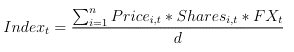
where

Price = Share price

Shares = number of outstanding shares

F Xt = the US$ exchange rate for the home country currency

t = time

i = individual index constituent member

d = the divisor which has been chosen to fix the value of the index at the starting date of 31st December 2023, equal to 1000. The divisor is adjusted to reflect changes in index constituents or capitalization events, to avoid any distortion to the index.

2.5 Investing in Stock Indices

While Kenny and Moss (1988) had previously hypothesized that stock markets improve the functioning of the domestic financial system in general and the capital market in particular, Singh (2022) found that stock markets are predicted to stimulate economic growth as they offer a boost to domestic savings. A list of well-known stock index investors together with the types of participation they engage in is shown in the table below.

Table 2.1: Investment in stock indexes

Types of Financial Institution	Participation in the stock markets
Commercial Banks	They issue stocks to boost their capital bases
Savings Banks	Invest in stocks for their investment portfolios
Insurance Companies	Invest premiums in the stock markets
Pension Funds	Invest a part of pension funds in the stock markets
Individuals	Invest their savings in shares to keep them afloat for future use

As a result, one must note that investing in stock indexes does not provide a guarantee about future financial prospects because of the stock markets’ erratic bullish and bearish behaviours.

2.6 Globalization of Stock Markets

Angel (2021), in accordance with portfolio diversification and optimization, investors can buy foreign equities, and businesses in need of capital can explore international markets. Studies have shown that stock investors can reap the rewards of foreign diversification, which not only helps with risk management but also spreads risk through risk sharing. Another important factor driving the globalization of stock markets is the urge to improve one’s reputation internationally. Due to the substantial benefits associated with the emergence of new financial products, particularly in the stock market’s derivatives sector, business volume has expanded; as a result, potential investors have strategically turned away from international risk. International stock trading was formerly halted by obstacles brought on by socio-political and technological divides, but these have since been lifted.

1. Reduction in transaction costs

Through computerization and improved telecommunications, many nations have integrated their stock markets, enhancing efficiency and lowering transaction costs. In order to facilitate the easy acquisition of stocks of European firms by investors in one country, the European markets have implemented a widespread cross-listing system known as Eurolist. In an effort to provide investors with a wider range of financial assets and to reduce trading costs, stock markets have formed strategic alliances, mergers, and consolidations as a result of increased competition.

2. Reduction in information costs

With the development of the Internet, investors can now access important information to make well-informed decisions without having to pay for it. International news and exchange rate updates provide important information for international investment, and countries are standardizing their accounting standards to facilitate the analysis and comparison of financial data. Investor security and confidence are provided at low information costs through bilateral agreements and decisions made by global governing bodies, like the G-8, regarding investment in poor countries.

3. Reduction in exchange rate risk

Supporting a single or common trading denomination, like the Euro, protects against this risk. As an alternative, agreements are being reached to use stable currencies, like the US dollar, in oil trade blocs like the Middle East. These agreements, along with restrictions on trading conditions, can help to advance the globalization of stock markets.

2.7 Challenges and Solutions to Developing Stock Markets

Because they are still in the early stages of development and have potential marketability due to their colonial ties, developing country markets present a strong platform for investment opportunities. Developing markets nevertheless encounter a few obstacles despite these potential benefits. Poor data management and storage limits the quantity of information available to investors for decision-making, particularly when it comes to financial data. As a result, a lot of trading and decision-making are based on conjecture and rumour. Because there are few shares available to other companies, the markets are tiny and extremely volatile.

As a result, huge transaction volumes regularly cause the equilibrium prices to jump, leaving them vulnerable to manipulation by powerful traders. Additionally, because it is hard to police laws and regulations against insider trading, it is more prevalent. During the 8th of February 2008 ADB Institute Symposium in Tokyo, Japan, the President of the Asian Development Bank emphasized the influence of international financial connections on market fluctuations. The performance of Asian markets would be impacted by the anticipated 1.5% slowdown in US economic growth in 2008, given the US’s substantial influence over global business cycles.

 Panic trading, which raises investor risk beyond what is thought to be beneficial, is often associated with periods of extreme political and social unrest. The nation of note is Cote d’Ivoire, where internal instability has discouraged potential investors from making investments. The majority of operations in African markets are completed manually, therefore trading infrastructure is lagging behind. However, Singh (1999) predicted that inadequate financial frameworks will cause these advancements to stumble. Investors’ alternatives for investments are limited due to the over-concentration of stock market activity on stocks, which restricts the range of items they can be exposed to.

 The extremely variable monetary policies in developing nations also affect stock market behaviour since inadequate liquidity tends to make investors less confident in the assets that are being offered. This can be linked to Swaziland’s 0.02% turnover ratio, which indicates that business is too low and that the market cannot support its operations on its own. It also indicates that there isn’t a strong local investor base. The free-float on African markets is often between 10 and 25 percent, which is extremely low by global standards and needs to be significantly revised in order to maintain competence. Significant economic issues, in addition to a lack of money and a large pool of jobless labourers, were the main obstacles to Ethiopia’s first stock market establishment, despite the country’s dire need for one.

A few strategies for advancing stock market development in underdeveloped countries and Africa include Automation, demutualization, attracting international involvement and institutional investors, regional integration, and tightening trade laws are some strategies for boosting stock markets in Africa and developing countries. In his statement, the president of the Asian Development Bank urged policymakers to continue pursuing sensible macroeconomic policies and to do tremendous effort to uphold confidence in their region. The issues of limited size and lack of liquidity can be resolved by cross-linking stock markets and removing exchange regulations while still preserving their unique national identities. This is the rationale behind the project’s inception, as we aim to comprehend the SADC stock markets’ reliance on one another for regional integration and expertise.

2.8 Shortcoming of Linear Correlation in Studying Dependence

Due to its ease of computation, manipulation under linear operations, and naturalness as a dependence measure in multivariate normal distributions as well as in general for multivariate spherical and elliptical distributions the majority of studies on dependence have focused on the linear correlation. According to Campbell, Lo, and MacKinlay (1997), its employment in the Arbitrage Pricing Theory (APT) and the Capital Asset Pricing Model (CAPM) demonstrated its significance in the theory of finance. Despite its widespread use, a number of studies, such as Embrechts et al. (1999), have demonstrated that it is inadequate for explaining dependence because of the influx of non-linear derivative products. This renders many of the underlying distributional assumptions invalid because it is not applicable to non-elliptical distributions. This is explained by Its sensitivity to outliers and the fact that it is only invariant under strictly increasing linear transformation are the reasons behind this. Due to the usual skewness and high tail of insurance claim data, these assumptions are invalid in the insurance industry.

Some of the recognized drawbacks of using linear correlation to gauge dependency include the following: Because heavy-tailed distributions, like the bivariate tv-distribution for v < 3, do not meet its criterion that variance be established between the variables of interest, non-life actuaries who model business losses with infinite variances are unable to draw important conclusions from it. Additionally, Cont (2001) demonstrated that a large number of financial and commodity price time series have the distributional feature of heavy tails, and so do not exhibit greater moments.

 Under the normalcy assumption, independence of two variables implies no correlation, however independence is not always implied by zero correlation. Given the well-known leptokurtic nature of commodity price data, the normalcy assumption is not particularly relevant.
Under non-linear strictly rising transformations T: < → <, that is, ρ(T(X), T (Y)) 6= ρ (X, Y), where X and Y are the random variables of interest, linear correlation is not invariant.

With elliptical distributions, a joint distribution can be created using the provided marginal distributions and correlation ρ value; however, this is generally not the case because the interval of possible correlation values gets smaller as data noise increases. In light of these constraints, alternative dependence measures such as copulas which are more adaptable to the constraints of linear correlation tail dependence, rank correlation, concordance measures, and tail dependence must be taken into consideration.

2.9 Copulas

A copula is a multivariate cumulative distribution function that is uniform across all marginal distributions on an n-dimensional cube when defined on [0, 1]. It describes the relationship between multiple variables, making it a useful tool for modeling dependences among them. The Latin word copulare, which meaning to join or connect, is the source of its name. The two parameters of interest in a copula are the weight parameter, which represents the shape of dependency, and the association parameter, which regulates the degree of dependence.

Families and types of copulas

Although there are many additional copula families in use, the Archimedean and elliptical copulas are the most significant copula families. Elliptical copulas model joint movements between variables, while Archimedean copulas model events when there is a lot of risk on individual stocks.

1. Elliptical copulas

The Student t-copula from the Student t-distribution, a derivative of the normal distribution, and the Gaussian copula, which are based on the normality assumption and typically serve as the standard for copulas, are found under the elliptical copulas. The Gaussian copula is referred to as a comprehensive copula because it is flexible enough to accommodate equal amounts of positive and negative dependence by incorporating both Frechet bounds within its acceptable range.

It can be represented as follows;

                                C Ga ρ (u1, u2) = ΦΣ Φ −1 (u1), Φ −1 (u2) 

where Σ is a 2 × 2 covariance matrix,

Φ is the cumulative distribution function of a standard normal distribution and

ΦΣ is the cumulative distribution function of bivariate normal distribution with zero mean and covariance matrix Σ.

The Student t-copula has two dependence parameters, ν (degrees of freedom) and θ (correlation), where ν controls the heaviness of the tails. The t-copula permits symmetric tail dependence and underestimates dependence when there is asymmetric dependence. It can be represented as follows;

                                  C t ν,Σ(u1, u2) = tν,Σ t −1 ν (u1), t−1 ν (u2) 

where Σ is a correlation matrix,

tν is the cumulative distribution function of the one dimensional tν-distribution and tν,Σ is the cumulative distribution function of the multivariate tν,Σ-distribution.

2. Archimedean copulas

Archimedean copulas are of the general form;

                                             C(u1, u2) = Φ−1

                                           (Φ(u1) + Φ(u2)) (2.9.6)

where Φ is a decreasing function mapping [0, 1] into [0, ∞] and it is called the generator

of the copula and this is well explained in the following theorem;

Theorem 2.3. Consider a continuous and strictly decreasing function Φ : [0, 1] :→[0,∞], with Φ(1) = 0, then

is a copula, if and only if Φ is convex.

Since they are simple to create, offer a large range of dependent structures, and have numerous parametric types of copulas that belong to them, Archimedean copulas are the most commonly used copulas. They are popular for modelling dependency across stock markets because they permit a larger dependence between extreme losses (such as when stock markets crash) than between extreme gains. The Product, Gumbel, Joe, Clayton, and Frank copulas as well as their combinations, such as the Clayton-Gumbel, are examples of Archimedean copulas.

When the distribution functions are continuous and the joint distribution is the product of the marginal, that is, H (x, y) = F(x), the product copula characterizes independent variables. G(y). The following equation provides the copula function for these two variables:

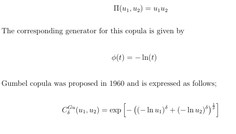
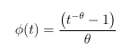
where δ ∈ (1,∞). For any value of δ, this copula does not reach the Frechet lower bound; values of 1 and ∞, on the other hand, correspond to independence and the Frechet upper bound. Gumbel shows very mild left tail dependency and substantial right tail dependence however it does not allow for negative dependence. Its generator is listed as follows;

If outcomes are known to be strongly correlated at high values (markets boom together), but less correlated at low values, then the Gumbel copula is an appropriate choice.

The Joe copula is similar to the Gumbel copula in that they both are suitable for modelling asymmetric dependence. The Joe copula is expressed as follows;

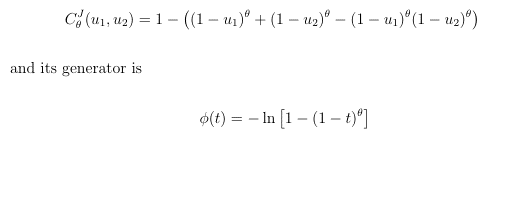
Clayton copulas were proposed in 1978 and are best described by the following equation;

The marginal become independent when θ → 0 and the copula attains the Frechet upper bound as θ → ∞ but cannot account for negative dependence. When correlation between two events is strongest in the left tail (markets crash together) of their joint distribution, Clayton copula is an appropriate modelling choice. The generator for this copula is given below;

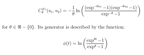
The other type of Archimedean copulas is the Frank copula shown below which exhibits no tail dependence because of its symmetry.

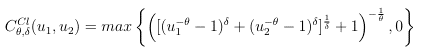
The ability of the Clayton-Gumbel copula to capture dependency in both tails allows it to describe asymmetric dependence. It is a hybrid of the Gumbel and Clayton copulas. Its formula, which goes by the name “Generalized Clayton copula,” is displayed below.

2.10 Copulas and Measures of Association

Rank correlation measurements have several characteristics, such as being dependent solely on the copula of the two random variables under study, being invariant under strictly increasing linear transformations, and being insensitive to outliers. This is important for formulating the underlying copula for modelling dependence, which is exemplified by the connection between Kendall’s τ and Archimedean copulas proposed by Genest and Mackay (1986). Therefore, the Kendall’s τ can be calculated using copulas as follows:

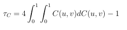
where C is the copula associated with the random variables, say (X,Y).

Spearman’s ρ is defined in terms of the copula associated with the random variables

as follows;

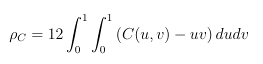
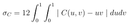
Schweitzer and Wolff’s σ can be computed in terms of copulas as follows;

Genest and Mackay (1986) showed that for Archimedean copulas, Kendall’s τ can be expressed in terms of the generator of the copula as follows;

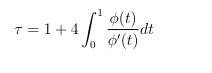
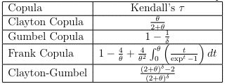
This was verified by Joe (1997) and hence, Kendall’s τ in terms of the association parameter θ for some Archimedean copulas are given in the table below;

Table 2.2: Kendall’s τ for some Archimedean copulas

2.11 Tail Dependence

This phenomenon, in particular, captures asymmetric correlation because multivariate time series data have extreme values. In a bivariate study, it is the likelihood that both of the variables being examined are at their extremes. The selection of copula to be used in dependence modelling is critically dependent on its existence. It can be captured by copulas within the dependence structure; the coefficients of the upper and lower tail dependence are of special significance. The coefficients of Archimedean copulas are obtained through the application of L’Hopital’s rule, as demonstrated by the following outcome:

Upper tail dependence means that given large values of u1, then large values of u2 31 are expected. Its coefficient is computed by the following equation;

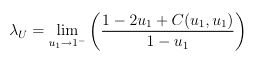
provided that the limit λU ∈ [0, 1] exists. The coefficient for the lower tail dependence is computed using the following equation;

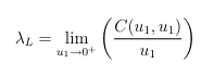
provided that the limit λL ∈ [0, 1] exists.

If λU > 0 or λL > 0, then we say that the two random variables under investigation have either upper tail or lower tail dependence.

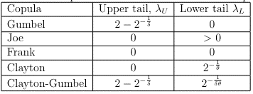
Since elliptical copulas are symmetric, we get λL = λU, which is greater than zero for the t copula and zero for the Gaussian copula. The existence of tail dependence in the data indicates that the Gaussian copula is incorrect, and the t copula is annulled by its asymmetric state. The following table lists the anticipated tail dependence levels for Archimedean copulas;

Table 2.3: Tail dependence levels for Archimedean copulas

2.12 Modelling Dependence using Copulas

The following are the advantages of using copulas in modelling dependence.

1. Offer an allowance to model both linear and non-linear dependence.
2. There is an arbitrary choice of the marginal distributions.
3. They are capable of modelling extreme data values.
4. They are invariant under increasing and continuous transformations. This property is very useful as transformations are commonly used in economics.

Copulas are extensively utilized in the fields of finance and economics, particularly in risk management and insurance, multivariate survival modelling, and bioinformatics. Understanding the interdependence of financial securities is crucial for managing portfolios, controlling risk clustering, pricing, and hedging. Here, the normalcy assumptions break out, which means that long-term business prospects may be compromised by investment decisions based solely on linear correlation.

Fitting copulas to data

Fitting copulas to data involves a number of methods, such as the maximum likelihood method, the inversion method, the empirical copula function (ECF), estimation using Kendall’s τ, and the inference function method for marginal (IFM). In this study, parametric copula estimation and copula parameter estimation from Kendall’s τ were the methods utilized to fit copulas to data. Because of the link between rank correlation coefficients and copulas and the relative simplicity of the computations, the former method is more attractive. The relations in Table 2.2 are utilized to calculate the parameters for the Archimedean copulas using this non-parametric method. Assessments of the goodness of fit are carried out using the Akaike Information Criterion, the Bayesian Information Criterion, and the Tests for goodness of fit are carried out using the log-likelihood statistics, the Akaike Information Criterion, and the Bayesian Information Criterion. Table 2.3 provides the relations that are used to compute the tail dependence levels.

The parametric two-stage estimation techniques and joint estimation are the two conventional methodologies that can be used for parametric copula estimation. Along with the copula, joint estimation entails estimating the marginal distributions of the two variables of interest. Because estimations of marginal distributions influence those for the copula, this results in misspecification error. The copula density is calculated using a given copula model and provided marginal distributions from

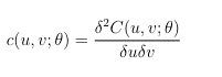
With respect to the copula density, random variable marginal densities, and marginal distributions, we derive the likelihood function for the paired observations. The copula parameter estimates are then obtained by maximizing the log likelihood function using the maximum likelihood technique. When there are too many parameters involved or when the marginal and copula both display complex forms, the limitations of this approach become clear.

 As the name implies, the two-stage parameter technique consists of two steps: first, the variables of interest are assumed to be independent, and their marginal distributions are computed parametrically using the log likelihood statistic. Following that, these are handled as nuisance parameters in the suggested copula model, and the maximum likelihood estimation method is applied right immediately.

These are thus regarded as nuisance parameters in the proposed copula model, and the estimation of the copula’s parameter estimations immediately employs the maximum likelihood estimation technique.

One parametric method that can be used to fit copulas to data is the maximum likelihood (ML) method. Due to the dependence structure’s emphasis in multivariate analysis, the dependence parameter must be margin-free; otherwise, parametric procedures yield estimates that are dependent on the margin. Therefore, applying the semi-parametric canonical maximum likelihood (CML) method would be a suitable substitute.

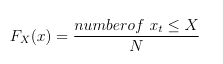
This method assumes no parametric form for the marginal distributions of the financial variables and estimates the copula’s association parameter. The benefit of this is that it is This approach has the advantage of being robust and allowing our conclusions to be free of distributional misspecification errors due to the non-specification of the underlying distribution. Say that a random variable’s empirical cumulative distribution function. X (which is an approximation of the true cumulative distribution function) is computed by the following formula;

Any two random variables can be used to convert a set of joint observations (Xt, Yt) of X and Y into a set of points (ut, vt) in the unit square by using the Probability Integral transform to define ut = FX(xt) and vt = GY (yt). The goal of CML is to maximize this data sets’ likelihood. Using both parametric and non-parametric two-stage approaches, this work aims to use copulas to simulate dependence across stock markets in five selected SADC nations, the profiles of which are provided in the next section.

2.13 Profiles of Stock Markets

The goal of this study was to analyse the mutual reliance among the five stock markets in the Southern African Development Community (SADC) in order to evaluate the potential for forming a potent regional trading bloc. The yearly US dollar returns for these stock markets as of February 12, 2024, are shown in Table 2.4 below.

 Table 2.4: Regional bourses Year-to-Date US$ returns: 12.02.24

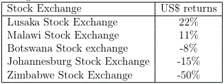
Shoprite, Zambia’s Sugar Company and the copper mine conglomerates are responsible for the outstanding performance of the Lusaka stock exchange. The ongoing blackouts of electricity and the depreciating value of the Rand as a result of the European securitization market closing provide insight into the downward trend of returns observed on the Johannesburg and Botswana stock exchanges. The market liquidity of the Zimbabwe stock exchange has been highly correlated, with substantial variances during events like the price blitz of March 2024. The subsections that follow provide brief summaries of various stock exchanges’ operational setups and performances.

1. Malawi Stock Exchange (MSE)

Established in March 1995, this came into operation in November 1996 under the close supervision of the Reserve Bank of Malawi. It started off with just one licensed broker and is now a fully functional stock market with both individual and corporate members. It uses a single price auction method and is governed by the Capital Markets Development Act (1990) and the Capital Market Development Regulations (1992). Traded products include government and equity securities. Foreign investment is limited to 5% of issued share capital for foreign investors, and as long as the investor is registered with the Reserve Bank of Malawi, there are no restrictions on capital repatriation. Weekly reports are used to share information since trading takes place throughout the working weekdays. There is no repository and settlement happens on a T + 7 basis, or seven days after the trade, with transaction clearing taking place.

2. Lusaka Stock Exchange (LuSE)

Zambia’s stock market was founded in 1994 with assistance from the World Bank’s International Finance Corporation in order to comply with the G-36 guidelines for the design and operation of the clearing and settlement system. Global custody services are provided by Barclays Bank of Zambia and Stanbic Bank of Zambia, which together make up the electronic depository facilities that make up the Central Share Depository. The Securities and Exchange Commission (SEC) was established as a result of the 1993 Securities Act, which regulates market activity. The majority of the listings on the LuSE, particularly in the mining industry, were impacted by Zambia’s privatization process. There are six stockbroking firms that are active on the market, and trade is mostly in government bonds and equities securities. Foreign investment is not banned.

3. Johannesburg Stock Exchange (JSE)

The main purpose of its establishment was to provide funding for the mining sector, which would increase employment and wealth generation. It is in the top ten largest markets worldwide and is the biggest stock exchange in Africa. It demutualized in July 2005 and now lists its shares on the Mainboard and AltX markets (which are for smaller, black-owned businesses). The Johannesburg Equities Trading (JET) system is used for order-based electronic trading of stocks, bonds, and derivatives. Transactions are carried out automatically when corresponding buy and sell prices are discovered. It was able to conduct trade with the Namibian Stock Exchange in 1998 by means of a communications link to the JET system. Insider trading is the primary obstacle to membership, which is available to both corporate entities and international individuals.

4. Botswana Stock Exchange (BSE)

Through Sechaba Investment Trust, which launched the country’s share market in June 1989, the Botswana Development Corporation (BDC) led public involvement in the country’s economy. Stockbrokers Botswana Limited, whose fees and commissions were set in accordance with rates from the Zimbabwe Stock Exchange, handled secondary market trading. To promote international investment, an Interim Stock Exchange Committee was established in October 1990. The Botswana Stock Exchange was fully founded in 1994 with the passing of the Stock Exchange Act. The Botswana Share Market Index is the only index that contains all listings. Ten percent of the market capitalization is made up of private investors, and foreign investment is limited to ten percent of a publicly traded company’s issued capital with limited funds repatriation. In general, it performs well.

5. Zimbabwe Stock Exchange (ZSE)

The Pioneer Column founded this in 1896, but it was subsequently put on hold because of the World Wars. The Zimbabwe Stock Exchange Act was first implemented in 1974 and was later changed in 1996 to become Zimbabwe Stock Exchange Act: Chapter 24:18. It was reaffirmed as the Stock Exchange Act upon Zimbabwe’s independence in 1980. It is composed of three indexes: Natfoods, the Zimbabwe Mining Index, and the Zimbabwe Industrial Index. There are over 65 listed securities, and corporations are prohibited from granting foreigners ownership of more than 40% of their shares.

MODEL, DATA AND METHODOLOGICAL FRAMEWORK

This study made use of real data that came from African Financial Markets. This database covers and keeps track of macro- and microeconomic financial market statistics for a few African countries. The stock indexes from five major markets in the SADC region Botswana, Malawi, South Africa, Zambia, and Zimbabwe constituted the data under inquiry. Over a period of almost four years, the study covered 565 trading days, or the trading dates from March 13, 2020, to March 4, 2024. The missing data values were attributed to improper data management and warehousing, as well as different technological barriers and national policies. These were regarded as randomly missing data. But the sampled information from the original database Nonetheless, the sampled data from the original database was adequate to draw reliable conclusions about the relationships without sacrificing their generality.

Using the statistical tool MINITAB, parametric estimating was carried out to find the marginal distributions that underlie each of the five stock markets. Based on the log-likelihood statistic and the Akaike Information Criterion (AIC), the best fit model was chosen. Based on these parameters, a class of competing models is narrowed down to the best model for explaining the stock market data. The study uses a log-linear model to evaluate the relationship between stock markets in small emerging economies.

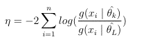
where ˆθk and ˆθL are the estimated parameters of the fitted and the true models respectively. The Akaike Information Criterion statistic is computed using the following equation;

where k is the number of fitted parameters in the model and η is the equivalent of the log-likelihood statistic. The selected model’s lack-of-fit is measured by the first term on the right-hand side of the above equation, and its growing unreliability as a result of its increased number of parameters is measured by the second term. The model with the lowest AIC among the rival models in the class is the best approximation model. Because the maximum likelihood function, which is unbiased and asymptotically effective, forms the basis of this test, it is reasonably reliable. For the data analysis in this study, the statistical programs MINITAB and R were utilized, and Latex was used for all typing.

RESULTS

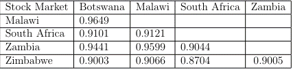
4.1 Correlation Analysis

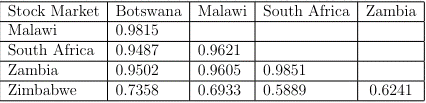
The existence of dependence between the stock market pairs was shown by a scatterplot matrix, which supported the necessity of performing a correlation analysis. Table 4.1 provides the correlation matrix pertaining to the five markets. Among the ten pairs, it is evident that the dependence between the markets of South Africa and Zambia is the strongest, while the dependence between the markets of South Africa and Zimbabwe is the weakest. With the exception of Zimbabwe, all other markets exhibited considerable interdependence, indicating both a high propensity for mutual growth and a greater prevalence of bullish traits. The fact that all other markets relied on the Zimbabwean market only sporadically could work against the leading efforts at regional integration.

Table 4.1: The linear correlation coefficients across stock markets

The non-parametric estimates of the Archimedean copula estimates were determined by computing the Kendall τ correlation coefficients, which are provided in Table 4.2. The strong Kendall τ correlation coefficients among the five stock markets in Table 4.2 can be attributable to their main characteristics: they are invariant under strictly increasing linear transformations and insensitive to the presence of outliers. This is also consistent with our contention that a different method needs to be taken into account when analysing the dependence structure among the five marketplaces that are being studied. There are outliers in the data for the Zimbabwe stock index, as seen by the significantly higher coefficients for Zimbabwe compared to all other markets in Table 4.2.

Table 4.2: The Kendall τ correlation coefficients across stock markets

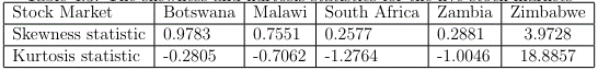
4.2 Nature of the Data and General Movement Patterns Across the Stock Markets

As can be seen in Table 4.3 below, all five stock markets have positive skewness statistics and negative kurtosis statistics, with the exception of the Zimbabwe Stock Market. Their magnitudes show that, with the exception of the Zimbabwean series all of the series had short, thin right tails and were therefore mainly non-peaked. These suggest that the data were skewed, therefore using elliptic distributions to explain them would be incorrect. The positive skewness statistics also show that the markets are primarily exhibiting bull run behaviour, which indicates that a flurry of active trading is taking place there.

Table 4.3: The skewness and kurtosis statistics for the five stock markets

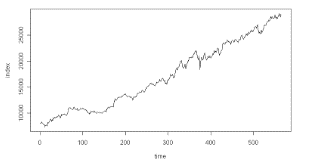
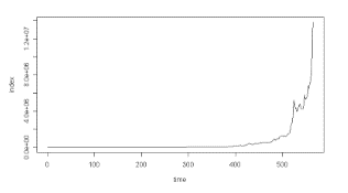
Most time series plot of the index data for the stock markets showed rising tendencies; the South African market’s and Zimbabwe’s in particular, which inclined more toward an exponential curve, is a prime example. Based on the plots, it can be concluded that the index data were generally rising gradually over time.

Normality Testing

Given that the Jarque-Bera statistic is known to asymptotically follow the chi-squared distribution with two degrees of freedom at the designated level of significance, Jarque-Bera test statistics were computed for each stock market to validate the assumption that the series exhibited the normal distribution. The decision was made at the significance level of 5%. Therefore, the calculated Jarque-Bera statistics were compared to χ 22 (0.05) = 5.99 for the five stock markets listed below.

Table 4.4: The Jarque-Bera test for normality for the five stock markets

Since the Jarque-Bera statistics were statistically significant, the null hypothesis that the stock market data followed a normal distribution was rejected. Using a non-parametric test for normalcy, the normality assumption was also disproved, and the outcomes are displayed below.

Table 4.5: The Kolmogorov-Smirnov test for normality for the five stock markets

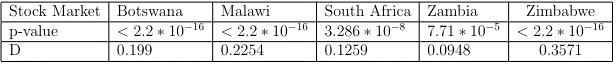
The series’ nonnormality was further demonstrated by the Kolmogorov-Smirnov test for normalcy. Given that the series’ values deviated statistically from zero, the D statistics showed that the empirical distribution functions for the series differed significantly from the normal distribution. The absence of outliers in the studied series or the manifestation of non-linearity characteristics in these series were both brought to light by the rejection of the null hypothesis of normalcy.

4.3 Non-Parametric Estimation of Copulas

On the basis of their relationships with the Kendall τ correlation coefficients, three different kinds of Archimedean copulas were computed non-parametrically. The following table presents estimates for θ in the copulas of Clayton, Gumbel, and Frank.

Table 4.6: Estimates of the parameter (θ) for the Clayton copula models for dependence across stock markets

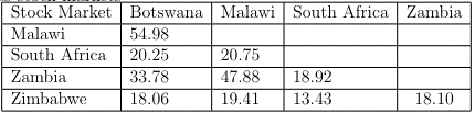
Table 4.7: Estimates of the parameter (θ) for the Gumbel copula models for dependence across stock markets

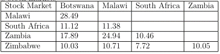
It was noted that the parameter estimates of the Clayton copula where almost twice the value of the estimates for the Gumbel copula.

Table 4.8: Estimates of the parameter (θ) for the Frank copula models for dependence across stock markets

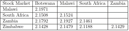
An estimate of the integral was utilized for the computation since the Frank copula formula for the estimation includes specific integrations like the Riemann Zeta function, which can be computed more precisely using MATLAB.

4.4 Tail Dependence

Examination Based on the parameter estimates for the Gumbel and Clayton copulas, respectively, from Kendall’s τ coefficients, tail dependency values were calculated at the significance level of 0.01 for both the upper and lower measures.

Table 4.9: Lower and (Upper) tail dependence values for all stock market pairs at α = 0.01

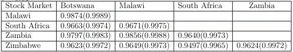
Significant indications of asymmetry tail reliance were found in every pair of stock market that was studied. Table 4.9 above showed that in all feasible stock market pairs, higher tail dependence was somewhat more pronounced than lower tail dependence. This indicates that large combined profits were more likely to occur in the stock markets than large combined losses.

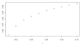
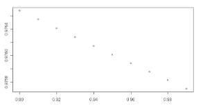
Lower tail dependence for the Gumbel copula     Upper tail dependence for the Gumbel copula

Figure 4.3 demonstrated how the lower tail reliance for the Gumbel copula approaches to zero when s→0, where s stands for the percentile points of risk. For every stock market, the values of upper tail dependency in figure 4.4 were nearly constant as s approached one, proving that the Gumbel copula is the most suitable model from non-parametric copula modelling. The Clayton copula’s suitability was not demonstrated by similar studies because lower tail dependency was not nearly constant across all stock markets. Therefore, the representation for the best fit copula estimation is as follows:

4.5 Parametric Distribution of the Stock Index Data (Marginal Distributions)

The most likely probability distributions that might explain the trends in the index data for the stock markets’ movement over time were found using MINITAB. The best model for all stock markets turned out to be the Extreme Value (Gumbel) distribution. This probability density function looks like this:

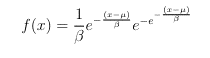
and its marginal distribution or cumulative distribution function is given by;

The estimates of the parameters of this model on the stock markets and their corresponding log-likelihood statistics(η) as well as their respective AIC were as tabulated below;

Table 4.10: Parameter estimates for the Extreme Value distribution for the stock markets

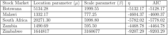
The Extreme Value distribution was the marginal distribution seen in all of the stock market index data. These were then used as nuisance parameters in the parametric selection of the most suitable copula models for the stock market pairs under investigation because copula models have the advantage of having the underlying marginal distribution for the data under investigation chosen arbitrarily.

4.6 Parametric Selection of Copula Models for the Stock Markets

Using the statistical program R, the maximum likelihood method was applied to find the best-fitting Archimedean copula models. According to Sklar’s Theorem (2.1), there are distinct copulas that describe the dependence structure for each pair of stock markets under study because all of the underlying marginal distribution functions for the stock markets were continuous. As can be seen in the table below, the Clayton copula best described 80% of the fits, while the Gumbel copula explained 20% of the fits. The best fit copula were identified using the Bayesian Information Criterion.

Table 4.11: Parameter estimates for the best fitted copulas for the stock markets

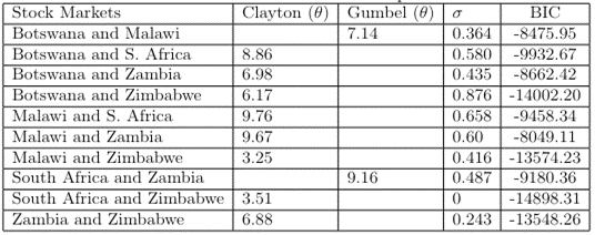
The Clayton copula is the most suitable copula for modelling reliance across these stock markets, according to the underlying distributions of the Extreme Value (Gumbel) distribution for the stock markets. Gaining a correct understanding of the tail behaviour of the data under study is one of the challenges in copula modelling. Parametric copulas might not be the best tool because the marginal misspecifications on the copula parameter estimation rely on the sign of skewness. According to Table 4.3, all of the skewness statistics for this study are positive, showing the existence of upper tail reliance. The skewness measurements indicate that the Gumbel copula is more appropriate because they show the presence of tail dependence in the data, which is a crucial measure in dependence modelling. In contrast, the parametric estimation results in Table 4.11 offset the bias in copula estimation to Clayton copula due to misspecification errors on the underlying distribution functions of the stock indices. The Gumbel copula, the best copula for non-parametric techniques, is appropriate because the behaviour of tail dependency in extreme circumstances determines how well the copula fits the data.

4.7 Comparison of the Estimates

According to the non-parametric and parametric estimate methods, the Gumbel and Clayton copula models, respectively, were the best fits. The non-parametric estimation findings were found to be more appropriate based on the goodness of fit approaches used. This is because tail dependency is a copula attribute, and using it in goodness-of-fit captures the largest skew present in the data. Since distributional misspecification errors produced marginal dependent estimates that involved complexity in the form of marginal distributions, it was not possible to exclude them from the parametric estimation.

CONCLUSION

Strong evidence of pairwise and mutual dependency across stock markets is used in this paper. With the exception of the Zimbabwe Stock Market, the five stock markets have strong correlation coefficients, suggesting that regional market integration is a viable endeavour. The fact that the markets tend to boom together with a better chance/probability than crushing together is supported by the strong levels of market concordance, which provides investors with a framework for portfolio diversification across markets. The data from the stock markets was highly skewed to the right and showed signs of non-normalcy. With the exception of Zimbabwe, whose index data jumped, the majority of stock market index data did not. According to the time series plots, all of the countries’ stock index series showed an upward trend, but the Zimbabwean market’s almost exponential spiralling value can be attributed to the high index values that resulted from hyperactivity on the money due to the availability of cheap money that needed to be disposed of quickly before it lost value.

All potential stock market pairs showed a strong degree of tail dependence, with a strong left- and right-tailed pattern. The stock markets were more likely to gain together than to lose together, according to the predominance of higher tail dependency over lower tail dependence. Therefore, for prospective investors looking to lower portfolio risk within these SADC stock markets, cross market diversification may be quite helpful. Stockbrokers, who support regional networking or partnerships among themselves and are leading the much-desired regional integration on informed grounds rather than just geographical accessibility, find great significance in this evidence of a high likelihood of right extreme co-movements. This demonstrated that the data was asymmetrically dependent rather than linearly dependent, which further supported the decision to ignore elliptical copulas in the modeling of the connection among different stock markets. The Extreme Value (Gumbel) distribution was the best suitable marginal distribution for characterizing the trend across all index data. This demonstrated that the Gumbel copula was suitable for characterizing the fundamental dependence structure of the data. We find that the markets tend to boom together because the Gumbel copula shows substantial right tail dependence, which is beneficial for investors looking to diversify their portfolios. The Gumbel and Clayton copulas, which represent the non-parametric and parametric estimations, respectively, were the most suitable Archimedean copulas to characterize the pairwise dependence structure among the five stock markets. Because tail dependency is a copula feature, misspecification errors caused by the underlying marginal distributions used in parametric estimation gave non-parametric estimation an advantage over the latter in inference. Therefore, the dependence between the stock markets was better explained by the non-parametric estimation. Based on non-parametric estimate, the Gumbel copula provided a more adequate explanation of the stock market’s dependency. As a result, the markets often grow in tandem, which is advantageous for portfolio diversification but should be approached cautiously by local investors.

REFERENCES

1. Quesada-Molina J.J(2003), What are copulas? Monografias del Semin. Matem. Garcia de Galdeano. 27: 499-506,
2. Hopkins, K.D. and Weeks, D.L. (1990), Tests for normality and measure of skewness and kurtosis: Their place in research reporting. Educational and Psychological Measurements, 50, 717-729
3. DeCarlo, L.T. (1997), On the meaning and use of kurtosis. Pschological Methods,2, 292 307
4. Lee Ruben (1998), What is an exchange?: The automation, management, and regulation of financial markets, Oxford University Press Inc., New York
5. Embrechts,P., A. McNeil and D. Straumann(2002) Correlation and dependence in risk management: properties and pitfalls, Risk Management: Value at Risk and Beyond, ed. M.A.H. Dempster, Cambridge University Press, Cambridge,pp 176-223.
6. Embrechts,P., Lindskog, F., McNeil A. (2003) Modelling dependence with copulas and applications to risk management,In Handbook of Heavy Tailed Distributions in Finance, ed. S. Rachev, Elsevier, Chapter 8, pp. 329-384. Also available at: www.math.ethz.ch/ baltes/ftp/papers.html Pranesh Kumar and Mohamed M Shoukri (2007) Copula based prediction models: an application to an aortic regurgitation study. BMC Med. Res. Methods. 7:21, Published online 2007 June, 6-doi:10.1186/1471-2288-7-21
7. Johnson, Timothy E (1978), Investment principles., Englewood Cliffs, New Jersey: Prentice Hall Tessema A. Prospects and challenges for developing securities markets in
8. Ethiopia: An analytical review: African Develpment Review, Volume 15, Number 1, June 2003, pp. 50-65(16) Blackwell Publishing. http://www.investopedia.com/university/indexes
9. Charles amo Yartey and Charles Komla Adjasi,2007. “Stock markets development in Sub-Sahara Africa: Critical issues and challenge” IMF Working Paper 07/209, International Monetary Fund
10. Jeff Madura (2001) Financial markets and institutions, 5th ed. Ohio, Southwestern College Publishing, Thomson Learning
11. Patton,A. J., 2007, Copula-based models for financial time series, In T. Andersen, R. Davis, J.P. Kreiss, and T. Mikosh, editors, Handbook of Financial Time Series. Springer Verlag.
12. Nicoloutsopoulos, D. (2005), Parametric and Bayesian non-parametric estimation of copulas, Ph.D thesis, University College London
13. Kpanzou, T. A (2007), Copulas in Statistics, PGD thesis, African Institute for Mathematical Sciences (AIMS)
14. Mutua,F.M.(1994), The use of Akaike Information Criterion in the identification of an optimum flood frequency model, Hydrological Sciences Journal,39(3):pp.235 – 244
15. Longin F, and B. Solnik (2001), Extreme correlation of international equity markets, Journal of Finance, 56(2):pp. 649 – 676
16. Hu, L(2002), Dependence patterns across financial markets: Methods and Evidence, Manuscripts, Yale University