
Lapsation Logistic Regression Model: A Case in Life Insurance
- Siti Nurasyikin Shamsuddin
- Sarahiza Mohmad
- Nur Haidar Hanafi
- Muhammad Hilmi Samian
- Diana Juniza Juanis
- Iylia Nadhirah Zahir
- 4179-4190
- Aug 16, 2025
- Economics
Lapsation Logistic Regression Model: A Case in Life Insurance
Siti Nurasyikin Shamsuddin, Sarahiza Mohmad, Nur Haidar Hanafi*, Muhammad Hilmi Samian, Diana Juniza Juanis, Iylia Nadhirah Zahir
Faculty of Computer and Mathematical Sciences, University Technology MARA, Malaysia
*Corresponding author
DOI: https://dx.doi.org/10.47772/IJRISS.2025.907000339
Received: 10 July 2025; Accepted: 17 July 2025; Published: 16 August 2025
ABSTRACT
Life insurance lapse poses significant financial challenges for insurers and policyholders, yet the determinants of lapse behaviour remain inconsistent across studies. This study identifies key factors influencing lapse prediction in life insurance contracts using logistic regression analysis on data from 499 policyholders in Malaysia. The analysis reveals that smoking status, payment mode, and face amount significantly impact lapse rates, while age and gender show no statistically significant influence. Smokers exhibit higher lapse odds compared to non-smokers, and quarterly premium payments correlate with increased lapse likelihood relative to monthly payments. Policies with lower face amounts demonstrate markedly higher lapse rates. The predictive model achieves 79.6% accuracy, underscoring its robustness in classifying lapse behaviour. These findings highlight the critical role of behavioural and financial factors over traditional sociodemographic variables in lapse prediction. The results provide actionable insights for insurers to design targeted retention strategies, such as flexible payment structures and tailored policy features, to mitigate lapse risks. Future research should expand the model to include additional variables like income and economic conditions to enhance predictive power. This study contributes to the literature by clarifying inconsistent findings and offering empirical evidence to refine lapse risk management in the life insurance industry.
Keywords: Lapse, Insurance Lapse, Life Insurance, Logistic Regression, Insurance Policy
INTRODUCTION
One important factor in fostering the socioeconomic growth of the modern economy is life insurance. When a person’s life is insured, an insurance company agrees to pay a payout upon that person’s death. One of the issues occurring in this industry is the lapsed policy. Both the insurance provider and the policyholder are impacted by a lapsed policy. High lapse rates make it more difficult for insurers to recover expenses incurred, such as significant underwriting charges and start-up expenses from sales costs and commissions. Publications on lapsed policies have increased since the 1990s, with socio-demographics and economics in the study analysis.
The behavioural interpretation offers unique insights into early lapses. High lapse rates hinder insurers’ ability to recoup upfront expenses (Eling and Kiesenbauer, 2014), while policyholders lose financial protection and forfeit premiums (Russell et al., 2013). Researchers have extensively studied lapse causes and modelling since the 1990s, examining behavioural characteristics, sociodemographic and economic factors (Eling and Kochanski, 2013). Behavioural interpretations highlight how decision-making processes and external factors influence policyholder behaviour (Dar and Dodds, 1989), yet findings remain inconsistent—particularly regarding sociodemographic variables like age, gender, marital status, smoking habits, payment methods, face amounts, dependents, and insurance types (Kuo et al., 2003).
In spite of a large amount of research on policy lapses, the effect of sociodemographic variables is inconsistent and not well investigated. For example, research yields conflicting evidence on age, gender and marital status effects (Kuo et al., 2003; Fang Wu, 2020). This study overcomes these gaps by considering behavioral and financial indicators—smoker status, payment method, and face amounts—to enhance predictive power and provide managerially beneficial insights for insurers.
These inconsistencies underscore policy lapse complexity and the need for further investigation. Contemporary economic conditions and evolving consumer behaviours provide opportunities to refine our understanding of lapse determinants. This study seeks to identify key factors influencing life insurance policy lapses, offering actionable insights for insurers to minimize lapse rates. Furthermore, it provides evidence-based recommendations to strengthen the life insurance framework, benefiting both industry and policyholders.
LITERATURE REVIEW
A lapse occurs when a policyholder terminates an insurance policy, often due to non-payment of premiums, impacting insurers’ financial stability (Shamsuddin et al., 2022). Lapse rates, defined as the fraction of terminated policies in a specific period, highlight the risk of loss from policy terminations and renewals. Modern research emphasizes the evolving significance of lapse behaviour, with economic factors and non-forfeiture provisions influencing policyholders’ decisions (Grosen & Jørgensen, 2000; Michorius, 2011).
Policyholders’ Lapse Prediction
Lapse rates depend on multiple factors, including policy type, duration, and economic conditions. Higher market interest rates increase lapse rates as policyholders seek better financial opportunities (Milhaud et al., 2010). Socioeconomic challenges, dissatisfaction with pricing, and shifting priorities drive policy terminations, reducing insurers’ renewal rates (Zhang, 2020). The interplay of these factors demonstrates that lapses arise from a complex combination of individual and market influences.
Based on the review of the literature, it can be seen that sociodemographic and behavioural variable interaction is infrequently reported in the literature. Others, on the other hand, look at the impact of elements like age and the gender of people or limitations on behaviours, the financial ones (Barsotti et al., 2016; Ho et al., 2012). These confusions suggest the need for integrative models, such as models that account for individual differences and environment. The relationship between payment options and lapse rates has brought to light the importance of financial flexibility which, in turn, seems to have overcome the effects of sociodemographic ones. Steps to bridge these gaps will further the development of predictive models and provide indications for targeted interventions to reduce lapsation.
Age
Age is a critical determinant of lapse rates, with younger policyholders showing higher lapses due to economic constraints (Barsotti et al., 2016). Research indicates that policies issued to individuals under 20 exhibit similar lapse rates to older age groups due to premiums often being paid by family members (Fang & Wu, 2020). Lapse rates generally improve with age, except for younger policies, where financial challenges are prevalent (Mojekwu, 2011).
Gender and Face Amount
Gender and face amount influence policy lapses, with females demonstrating better long-term persistence than males, despite slightly higher early lapse rates (Fang & Wu, 2020). Policies with lower face amounts show higher lapse rates, while larger face amounts exhibit modest variations (Actuaries, n.d.). On average, males have higher face amounts, but financial prudence among females contributes to better policy adherence (Purushotham, 2006). These factors underscore the combined effect of gender and face amount on lapse patterns.
Smoking Status
Smokers and non-smokers are treated differently in life insurance pricing. Usually, smokers tend to face higher premiums compared to non-smokers policyholders due to higher risk and mortality rate (Sari et al., 2019). According to Verisk Analytics, Inc., a data analytics and risk analysing firm, life insurers lose premiums worth an estimated RM3.4 billion a year as a result of tobacco consumption that is not declared upfront in an insurance contract. Therefore, it is important to identify smoking status during the underwriting process. Ho et al. (2012) stated that smokers and non-smokers exhibited similar rates of lapsation by year with non-smokers lapsing slightly more often than smokers in the early years and the opposite trend in later years in whole life insurance. However, for terms insurance plans, smokers lapsed more often than non-smokers at all policy duration. This is due to the fact that pricing is frequently the most important factor in both purchasing and keeping insurance coverage. Smokers might have discovered more affordable smoking rates through new product offerings, or they might have felt that their plans were too costly to maintain. For investment link products such as variable universal life plans, the lapse rate is constant between smokers and non-smokers mainly because it is still new on the market.
Payment Mode
According to Fang and Wu (2020), the lapse rate generally increases with the number of premium payments made annually in whole life policy. Policies that are paid directly each month using an electronic fund transfer method are an exception to this regulation. There are several different premium payment methods, including monthly, quarterly, semi-annual, and annual payments. Jayetileke et al. (2017) found that mode of payment has a highly significant factor for the persistence of life insurance policies. For the studies shown that the monthly paying mode has higher frequency. It is a key variable in keeping the policy in force longer than the other mode of payments. Koijen et al. (2022) found that during recession young policyholders who live in lower-income areas and have higher health risks are more likely to lapse their policies. Ho et al. (2012) stated that the lapse rates in policy with annual premium payment mode are lower than other payment mode in whole life policy. While in term life policy, quarterly payments result in the highest lapse rate compared to monthly payment.
Face Amount
Face amount of life insurance refers to the total sum of money that the insurance company agrees to pay upon the death of the insured or at the policy’s maturity. It can also be referred to as the death benefit or the face amount of life insurance. According to Ho et al. (2012), term insurance face amount lapse rate has decreased significantly due to the increase of guaranteed level premium term policy. While in whole life insurance, experience higher lapse rates during early policy years due to higher premium. Actuaries (n.d.) discovered that the majority of values, differences by face amount are rather small. Larger policies, however, show more lapses than average. According to policy, 60% of the population in the whole life sample is male and 40% is female. Males have an average face amount of RM40,000, while females have an average of RM26,000. Lapse rates showed a more even trend by policy year, with early-year policies having lower face-amount lapse rates and later-year policies having greater face-amount lapse rates. Policyholders with smaller face amounts had greater lapse rates on a face amount basis.
METHODOLOGY
This section outlines the research methodology employed in this study, detailing the data sources, theoretical framework, and analytical methods. The analysis primarily relies on logistic regression, a statistical approach widely used for binary outcome predictions and classification tasks.
Sources of Data
This research utilizes secondary data, defined by Hox and Boeije (2005) as data obtained from existing sources where variables are pre-coded with a range of values. Such datasets, often comprising quantitative and qualitative elements, provide a rich basis for analysis. For this study, data was sourced from an insurance company in Malaysia, encompassing 499 policyholder records. This study adhered to ethical guidelines in using secondary data. All policyholder information was anonymized, and data access was limited to the research team to ensure confidentiality. Data use was formally consented to by the insurance company, thus ensuring ethical treatment of policyholder data.
The dataset includes six variables selected based on prior literature: age, gender, smoking status, payment mode, face amount, and lapse prediction. These variables are recognized as common predictors in research concerning policy lapse behaviour. Although additional variables could be explored, this selection ensures consistency with established studies. Table 1 below shows the descriptions of variables.
Table 1. Descriptions and Coding of Predictor Variables
| Variable Name | Variable Type | Description |
| Age | Categorical | Age in years.
1 : 30 and below 2 : 31-40 3 : 41-50 4 : 51 and above |
| Gender | Nominal | 1 : Male
2 : Female |
| Smoking Status | Binary | 1 : Smoker
2 : Non-smoker |
| Payment Mode | Binary | 1 : Quarterly
2 : Monthly |
| Face Amount | Categorical | 1 : RM100 and below
2 : RM101-RM300 3 : RM301 and above |
| Lapse in Life Insurance Contract | Binary | 0 : Not lapse
1 : Lapse |
Theoretical Framework
The theoretical framework as shown in Figure 1 conceptualizes lapse prediction as dependent on key demographic and policy-specific factors, namely age, gender, smoking status, payment mode, and face amount.
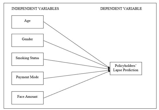
Figure 1. Theoretical Framework for Lapse Prediction in Life Insurance Contracts
Descriptive Analysis
Initial analysis involves a demographic breakdown of the dataset, summarized using frequency tables. This step provides a foundational understanding of the variable distributions.
Logistic Regression Analysis
The data analysis in this study employs Logistic Regression, also known as the logit model, which is widely recognized for its effectiveness in classification and predictive analytics. According to IBM Technology Corporation, Logistic Regression estimates the likelihood of a specific outcome, such as “yes” or “no,” based on a given set of independent variables. Since the model outputs probabilities, the dependent variable’s range is restricted between 0 and 1. This method not only assesses the significance of predictors but also determines the direction of their associations, whether positive or negative.
As noted by Park (2013), Logistic Regression is particularly suitable for situations where the dependent variable is binary. Similar to other regression analyses, Logistic Regression serves as a predictive tool to describe and analyze the relationships between one binary dependent variable and one or more independent variables that can be nominal, ordinal, interval, or ratio-scaled.
Given that the dependent variable in this study—policy lapse prediction—is binary, Logistic Regression is an appropriate analytical method. This approach is crucial for managing the complex relationships among the various factors influencing lapse prediction, including policyholders’ age, gender, smoking status, payment mode, and face amount. By systematically evaluating these variables, Logistic Regression identifies the most significant predictors and determines their relative impact on the likelihood of a policy lapse. This comprehensive analysis provides valuable insights for understanding and addressing policyholder behavior.
The logistic regression model is expressed as:
logit(p)=ln(p/(1-p))=β0+β1 X1+β2 X2+β3 X3+β4 X4+β5 X5
where:
p = Probability of lapse
β0 = Intercept
β1, β2,…,β5 = Coefficients for predictors
X1, X2,…,X5 = Predictor variables (e.g., age, gender)
Model Validation and Assumptions
To ensure the validity of the logistic regression model, it is essential to verify model adequacy. This involves confirming the absence of multicollinearity among the predictor variables, which ensures that the independent variables are not highly correlated, preserving the reliability of the regression coefficients. Additionally, the model should be free from strongly influential outliers, as such data points can disproportionately affect the results and lead to biased or unreliable conclusions. These checks are critical for maintaining the robustness and interpretability of the logistic regression analysis.
Hosmer and Lemeshow Test
It is a test of goodness-of fit, where to determine whether the data is good fit for the logit model or not.
H0: The logistic regression model is a good fit for the data.
H1: The logistic regression model is a poor fit for the data.
The model is good fit for the data if p-value is greater than α = 0.05
Omnibus Test
The test is conducted by comparing the model containing the predictors to a null model, which excludes all predictors. If the p-value is less than the significance level α = 0.05, it indicates that the inclusion of the independent variables significantly improves the model’s ability to predict the dependent variable. This outcome demonstrates that the independent variables provide valuable information for explaining variations in the dependent variable.
Cox and Snell R Square and Nagelkerke R2
It provides an indication of the amount of variation in that predicted variable explained by the model.
The value range: 0 < R2 < 1
Classification Table
The proportion of individuals within the group possessing the characteristic of interest is quantified through sensitivity, which measures the true positive rate. Conversely, specificity evaluates the true negative rate, representing the proportion of individuals without the characteristic of interest. These metrics are essential for assessing the model’s accuracy in distinguishing between the presence and absence of the characteristic.
Model Evaluation
H0: There is no significant relationship between the independent variable and the dependent variable.
H1: There is a significant relationship between the independent variable and the dependent variable.
The statistical significance of the model is evaluated using the Chi-Square test. This involves comparing the calculated p-value against a predefined significance level α = 0.05. If the p-value is less than α, the model is considered statistically significant, indicating that the predictors collectively contribute meaningfully to explaining variations in the dependent variable.
Summary of Data Analysis
This study includes quantitative data analysis that was conducted using IBM SPSS version 29. The findings will be presented descriptively, using pie charts to illustrate key aspects. Logistic regression was employed to assess the influence of multiple predictor variables on the outcome variable, enabling a deeper understanding of how each factor contributes to the results. This analytical approach enhances the accuracy and precision of the findings, providing valuable insights into the relationships between variables. As this study utilized secondary data, obtaining permission and consent for data collection was crucial. Before beginning the data collection process, a formal request letter was submitted to the target company, as previously mentioned.
RESULTS AND ANALYSIS
This section discusses the results from descriptive analysis, tests for several model evaluations for logistic regression, such as the Omnibus Test of the Model Coefficient, the Hosmer-Lemeshow Test, Cox and R-square, and the Nagelkerke R-square, and Logistic Regression’s output. The goal is to identify factors that contribute to lapse prediction in life insurance contracts. To analyze the data, IBM SPSS version 29 will be used to compute the results for all tests mentioned above.
Descriptive Analysis
The lapsed status was used as the dependent variable in predicting the life insurance lapse, with 39.1% of the total policyholders having lapsed their policies, as shown in Table 2. Almost half of the policyholders were aged 30 years and below, at 49.5%, followed by those aged 31 to 40 years old and 41 to 50 years old, with 37.3% and 9.2%, respectively. Meanwhile, the policyholders who are aged 51 years old and above are the lowest, with only 4% of the policyholders. Out of 499 policyholders, 56.3% are males, 57.3% are not smoking, and 67.7% made a monthly premium payment. Most of the policyholders have a face amount of RM100 and below, followed by RM101 to RM300, with 46.1% and 45.1%, respectively. Meanwhile, only 8.8% of them have a face amount of RM301 and above.
Table 2. Frequencies of Variables
| Variables Name | Description | Frequency | Percentage |
| Age | 1 = 30 years old and below
2 = 31 – 40 years old 3 = 41 -50 years old 4 = 51 years old and above |
247
186 46 20 |
49.5
37.3 9.2 4.0 |
| Gender | 1 = Male
2 = Female |
281
218 |
56.3
43.7 |
| Smoking Status | 1 = Smoking
2 = Not Smoking |
213
286 |
42.7
57.3 |
| Payment Mode | 1 = Quarterly
2 = Monthly |
161
338 |
32.3
67.7 |
| Face Amount | 1 = RM100 and below
2 = RM101-300 3 = RM301 and above |
230
225 44 |
46.1
45.1 8.8 |
| Lapse | 1 = Not lapse
0 = Lapse |
304
195 |
60.9
39.1 |
Model Evaluation of Lapse Prediction
Prior to running logistic regression, model adequacy checking was performed. Table 3 shows the absence of multicollinearity because the Variance Inflation Factor (VIF) value is less than 10 for all predictor variables. Tolerance is the reciprocal of the Variance Inflation Factor. A tolerance value of less than 0.2 indicates multicollinearity. Thus, this study shows the absence of multicollinearity because the tolerance value for all predictor variables is more than 0.2.
Meanwhile, the outliers in Y were checked based on the studentized deleted residuals. Observation that has more than 3 for the value of studentized deleted residuals is considered an outlier. In this research, all studentized deleted residual values in Y are less than 3. After removing the outliers, the results obtained are still the same. Hat Matrix Leverage Values are used to check the outlier in X, and the cutoff point is 0.024. A high leverage value indicates a leverage point or an outlying case with regard to the X values. There are only a few outliers in X, which are on Observation 28, 230, and 435. Other than that, most of the leverage value of the 499 observations is less than 0.024.
Table 3. Multicollinearity Diagnostics: Tolerance and VIF Values
| Variables | Tolerance | VIF |
| Age | 0.908 | 1.101 |
| Sex | 0.477 | 2.095 |
| Face Amount | 0.748 | 1.337 |
| Payment Mode | 0.795 | 1.259 |
| Smoking Status | 0.476 | 2.101 |
The results of the model evaluation test based on the Omnibus Test for Model Coefficient, Hosmer-Lemeshow Test, Cox and R-Square, and Nagelkerke R-Square are summarized in Table 4. According to the Hosmer-Lemeshow Test, the estimated model for the first model fits the data as the null hypothesis of this logistic regression model is a good fit for the data and is accepted at a 5% level. Furthermore, the Omnibus Test of Model Coefficient results suggest that independent variables better predict the dependent variable as the test is significant at a 5% level. By looking at the Cox and R-Square and Nagelkerke R-Square values, the variability of the dependent variable is between 34.3% and 46.5% can be explained by the overall model.
Table 4. Goodness-of-Fit Statistics for Nested Logistic Regression Models
| Tests | Model 1 | Model 2 | Model 3 |
| Omnibus Test of Model Coefficient | 0.000 | 0.000 | 0.000 |
| Hosmer and Lemeshow Test for Goodness of Fit (p-value) | 0.688 | 0.226 | 0.893 |
| Cox and Snell R-Square and
Nagelkerke R-Square |
0.343
0.465 |
0.343
0.465 |
0.341
0.462 |
Based on Table 5, Model 2 shows that after dropping the Gender variable, the Logistic Regression Model also fits the data with a p-value of 0.226. For the Omnibus Test of Model Coefficient, results suggest that the information from predictors in Model 2 allows for better prediction of the outcome as the null hypothesis is rejected at the 5% level. Moreover, the values of Cox and Snell R-Square and Nagelkerke R-Square for Model 2 are 0.343 and 0.465, respectively, which is similar to Model 1. This suggests that the variability in lapse prediction in life insurance contracts is 34.3%, and 46.5% can be explained by the overall model.
The dropping of the variable Age for Model 3 gives a similar result since the p-value of the Hosmer and Lemeshow Test is more than 0.05. For the Omnibus Test of Model Coefficient results, the p-value is less than 0.05, suggesting information from predictors in Model 3 allows for better prediction of the explanatory. Interestingly, the three variables (Smoking Status, Payment Mode, and Face Amount) give a better prediction for this model after Gender and Age as unimportant variables are dropped from the model. For this model, both R-squared values indicate the total variation of the factors affecting the lapse prediction in life insurance contracts, which is about 34.1% and 46.2%, as explained by all factors included in the model. In conclusion, the results from this section show that Model 3 is the most significant model.
The sensitivity of model 3 is 80.3%. This means that the model correctly classifies 80.3% of the insurers who have not lapsed. Next, the specificity is 78.5% of insured who are lapsed. It can be concluded that predictive models are more powerful in predicting Y=0 than Y=1. It is based on a higher sensitivity rate than the specificity rate. Since the overall percentage is 79.6% more than 50.0%, then the model possesses good predictive efficiency. Table 3 shows the p-value for each independent variable in the logistic regression model.
Table 5. Predictor Significance Across Sequential Models (p-values)
| Variables | Model 1 | Model 2 | Model 3 | |||
| Variable | P-Value | Variable | P-Value | Variable | P-Value | |
| Included
Variables |
Age | 0.266 | Age | 0.233 | Smoking Status | 0.000 |
| Gender | 0.752 | Smoking Status | 0.000 | Payment Mode | 0.000 | |
| Smoking Status | 0.000 | Payment Mode | 0.000 | Face Amount | 0.000 | |
| Payment Mode | 0.000 | Face Amount | 0.000 | |||
| Face Amount | 0.000 | |||||
Note 1: 0.000 indicates p value < 0.001
In finding the most contributed variables for the model, all independent variables, which are Age, Gender, Smoking Status, Payment Mode, and Face Amount, are included in the full model (Model 1). Three variables contribute to the first model: smoking status, payment mode, and face amount, as the null hypothesis of Wald statistics is rejected at a 5% level of significance. Meanwhile, the other two variables, Age and Gender, do not significantly contribute to the model with a p-value of more than 0.05. Thus, the variable with the highest p-value is dropped from the model, which is Gender. Gender is the least important variable that contributes to the model.
Despite age and gender being suggested as the main predictors of policy lapsing as in previous studies (e.g., Barsotti et al., 2016; Mojekwu, 2011), the inadmissible age and gender in the present study can be explained by the homogeneity of the sample, or the greater weight given to behavioural and financial determinants. Results are in line with previous work suggesting that smoking status, payment modes, and face amount are frequently the leading sociodemographic predictors of sociodemographic factors in predictive modeling (Fang Wu, 2020). Future research could investigate this by comparing different population samples to determine whether age and gender are truly contextually consequential.
For Model 2, the variables included are Age, Smoking Status, Payment Mode, and Face Amount. Variable Age still does not contribute to the model because the p-value for the variables is more than 0.05. Thus, the variable Age is dropped from the model because it has the highest p-value. Therefore, Model 3 is computed with three variables: Smoking Status, Payment Mode, and Face Amount. After running the model, the p-values for Smoking Status, Payment Mode, and Face Amount are less than 0.0,5, so those variables are kept in the model. Therefore, the final model, which is Model 3, consists of only variables: smoking status, payment mode, and face amount. This is because the p-value for the three variables is less than 0.05. This implies that there are three variables that significantly contribute to lapse prediction in life insurance contracts. Table 6 shows the best logistic regression model for lapse prediction in life insurance contracts.
Table 6. Final Logistic Regression Model Estimates for Lapse Prediction
| Variable | Estimate (B) | p-value | exp(B) |
| Constant | 0.035 | 0.916 | 1.035 |
| Smoking Status | -1.135 | **** | 0.321 |
| Payment Mode | -1.404 | **** | 0.246 |
| Face Amount | 1.433 | **** | 4.190 |
Note 2: **** indicates p-value < 0.001
Table 7. Confusion Matrix Table
| Actual / Predicted | Not Lapsed | Lapsed |
| Not Lapsed | 244 (TN) | 60 (FP) |
| Lapsed | 42 (FN) | 153 (TP) |
Note 3: Overall Accuracy: 79.6% (Sensitivity = 80.3%; Specificity = 78.5%)
The estimated best model based on the logistic regression is as follows:
Logit[P(Y = 1)]= 0.035−1.135SmokingStatus–1.404PaymentMode+1.433FaceAmount
where Y = 1 indicates the person who lapsed. The finding shows that the estimated coefficient for smoking status towards lapse prediction is negative (effect), the estimated coefficient for payment mode towards lapse prediction is negative (effect), and the estimated coefficient for face amount towards lapse prediction is positive (effect), which indicates that people who pay face amount contributed significantly to lapse in life insurance contracts.
The odds ratio will be used to reflect the effects of the significant variables on the lapse status. The odds of policyholders’ lapse in life insurance contracts for smokers are 0.321 times more likely compared to policyholders not smoking. The odds of policyholders lapsing in life insurance contracts for quarterly payments is 0.246 times more likely compared to policyholders paying for monthly payments. Meanwhile, the odds of policyholders’ lapse in life insurance contracts for policyholders with a face amount below RM100 is 4.190 times more likely compared to the other.
Based on the results, the factors that most contribute to the lapse in life insurance contracts are Smoking Status, Payment Mode, and Face Amount. This is because the significance value for those three variables is less than =0.05. Therefore, the objective is achieved based on the analysis. Based on certain literature reviews, it was true that lapse rates for smokers were significantly higher than for non-smokers. This is because price is often the key consideration in the purchase and retention of a policy. Next, for payment mode, based on literature reviews, lapse rates were higher for monthly than quarterly premium policies. Finally, on a face amount basis, policyholders with lesser face amounts had higher lapse rates.
Behavioural and Market Interpretations of Key Findings
Smokers exhibited 3.12× higher lapse odds (OR=0.321; p<0.001), likely due to premium affordability issues. Smokers face 20-30% higher premiums (Sari et al., 2019), increasing financial strain during economic downturns. Quarterly payers lapsed 4.07× more often than monthly payers (OR=0.246; p<0.001), as lump-sum payments amplify cash flow burdens (Fang & Wu, 2020). Policies with face amounts ≤RM100 had 4.19× higher lapse rates – suggesting lower-value policies are perceived as disposable during financial hardship (Ho et al., 2012). These findings underscore how behavioural economics (e.g., present bias) and market design (e.g., payment flexibility) drive lapsation more than demographics.
CONCLUSION
In summary, this research aimed to present a thorough analysis of the body of knowledge regarding policy lapses in life insurance, emphasizing identifying the predictive variables that influence policy lapses. By investigating the effects of important characteristics, including age, gender, smoking status, payment method, and face amount, on lapse prediction in life insurance contracts, the study effectively met its goals.
The results show that smoking status, payment method, and face amount were the most significant factors influencing policy lapses out of the five categories studied. These findings imply that behavioural and financial factors, including smoking behaviours and the method and number of premium payments selected, greatly influence a policyholder’s likelihood of keeping coverage. Age and gender, on the other hand, were shown to have little to no impact on lapse prediction, suggesting that they may not be important in determining policyholder behaviour in this situation.
The predictive model established for this study showed a high degree of accuracy, with an overall predicted accuracy of 79.6%. This indicates that it is a good fit for determining and elucidating the main causes of policy failures. This strong performance demonstrates how useful the model is as a tool for insurers to comprehend and lessen policy lapses.
Insurers can strategically integrate these empirical insights into practical retention frameworks through three targeted approaches: First, by implementing risk-adjusted pricing models that offer smoking cessation incentives or tiered premium structures for quarterly payers to alleviate affordability barriers. Second, deploying behaviourally-triggered communications—such as automated payment reminders and personalized engagement campaigns—for high-risk segments (e.g., smokers and non-monthly payers) to pre-empt lapse intentions. Third, undertaking product portfolio redesign that converts lump-sum payment plans into phased instalment options while bundling low-face-amount policies (≤RM100) with value-added health riders, thereby enhancing perceived utility and reducing disposability during financial distress. Such interventions translate predictive analytics into concrete business actions that directly address the behavioural economics of lapsation.
These revelations will significantly impact the insurance sector. Insurance companies can create focused strategies to lower lapse rates by concentrating on the important elements found in this study. These strategies include designing policies that accommodate policyholders’ financial flexibility, addressing behavioural risks like smoking, and streamlining payment structures to improve affordability and convenience. The results also offer a useful starting point for future studies that aim to improve predictive models and investigate additional variables affecting policy failures in various cultural or economic contexts.
Future research could incorporate additional sociodemographic and behavioural variables, such as income level, marital status, educational attainment, and economic conditions, to capture a more comprehensive picture of factors influencing lapsation. Exploring these variables may help uncover nuanced patterns and provide a richer understanding of the determinants of life insurance policy lapses.
Limitations
This study used data from a single Malaysian insurer, limiting generalizability. Key variables like policyholder income, marital status, and macroeconomic conditions were unavailable. Future work should incorporate these to refine model accuracy. Additionally, the binary smoking variable (smoker/non-smoker) overlooks cessation efforts, which may modulate lapse risk
REFERENCES
- Actuaries, C. I. (n.d.). (Tech. Rep.).
- Barsotti, F., Milhaud, X., & Salhi, Y. (2016). Lapse risk in life insurance: Correlation and contagion effects among policyholders’ behaviors. Insurance Mathematics and Economics, 71, 317–331. https://doi.org/10.1016/j.insmatheco.2016.09.008
- Dar, A., & Dodds, C. (1989). Interest Rates, the Emergency Fund Hypothesis, and Lapse Rates. Journal of Risk and Insurance, 56(3), 415-433.
- Eling, M., & Kiesenbauer, D. (2014). What Policy Features Determine Life Insurance Lapse? An Analysis of the German Market. Journal of Risk and Insurance, 81(2), 241-269.
- Eling, M., & Kochanski, M. (2013). Research on Lapse in Life Insurance: What Has Been Done and What Needs to Be Done? Journal of Risk Finance, 14(4), 392-413.
- Fang, H., & Wu, Z. (2020). Life insurance and life settlement markets with overconfident policyholders. Journal of Economic Theory, 189, 105093. https://doi.org/10.1016/j.jet.2020.105093
- Grosen, A., & Jørgensen, P. L. (2000). Fair valuation of life insurance liabilities: The impact of interest rate guarantees, surrender options, and bonus policies. Insurance Mathematics and Economics, 26(1), 37–57. https://doi.org/10.1016/s0167-6687(99)00041-4
- Ho, C., S. Muise, N., LIMRA, & SOA. (2012). U.S. Individual Life Insurance Persistency A joint study sponsored by the Society of Actuaries and LIMRA. In soa.org. SOA. https://www.soa.org/globalassets/assets/Files/Research/Exp-Study/research-2007-2009-us-ind-life-pers-report.pdf
- Hox, J. J., & Boeije, H. R. (2005). Data collection, primary versus secondary.
- Jayetileke, H., Perera, S., & Jayasekara, L. (2017). Factors Affect for the Persistency of Life Insurance Policy in Sri Lanka: Empirical Evidence from the Life Insurance Policy Holders. Journal of Scientific and Engineering Research, 4(3), 47–53
- Koijen, R. S. J., Lee, H. K., & Van Nieuwerburgh, S. (2022). Aggregate lapsation risk. SSRN Electronic Journal. https://doi.org/10.2139/ssrn.4141196
- Kuo, W., Tsai, C., & Chen, W. (2003). An Empirical Study on the Lapse Rate: The Cointegration Approach. Journal of Risk and Insurance, 70(3), 489-508.
- Michorius, C. Z. (2011). Modeling lapse rates: Investigating the variables that drive lapse rates (Unpublished master’s thesis). University of Twente.
- Milhaud, X., Loisel, S., & Maume-Deschamps, V. (2010). Surrender triggers in life insurance: classification and risk predictions. Laboratory de Sciences Actuarielle et Financiere (Working Paper). http://docs.isfa.fr/labo/2010.1%28WP2120%29.pdf
- Mojekwu, J. N. (2011). Study of Modes of Exit of Life – Insurance Policy holders in Nigeria: Trends and Patterns. International Business Research, 4(3). https://doi.org/10.5539/ibr.v4n3p182
- Park, H. (2013). An Introduction to Logistic Regression: From Basic Concepts to Interpretation with Particular Attention to Nursing Domain. Journal of Korean Academy of Nursing, 43(2), 154. https://doi.org/10.4040/jkan.2013.43.2.154
- Purushotham, M. (2006). Us individual life persistency update. LIMRAs Marketfacts Quarterly, 25(1), 36.
- Russell, D. W., Gough, O., & Isaacs, E. B. (2013). Understanding Policyholder Behaviour in Life Insurance. Insurance Markets and Companies: Analyses and Actuarial Computations, 4(1), 24-34.
- Sari, D. J., Lestari, D., & Devila, S. (2019). Pricing life insurance premiums using Cox regression model. AIP Conference Proceedings. https://doi.org/10.1063/1.5132461
- Shamsuddin, S. N., Ismail, N., & Roslan, N. F. (2022). What We Know about Research on Life Insurance Lapse: A Bibliometric Analysis. Risks, 10(5), 97.
https://doi.org/10.3390/ risks10050097 - Zhang, P. (2020). Evaluating the Cost of a Lapse in Life Insurance and its Implications on Developing a Policyholder Retention Strategy for a Company.